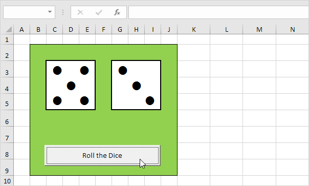
How to create Roll the Dice in Excel

This example teaches you how to simulate the roll of two dice in Excel.

Note: the instructions below do not teach you how to format the worksheet.

We assume that you know how to change font sizes, font styles, insert rows and columns, add borders, change background colors, etc.

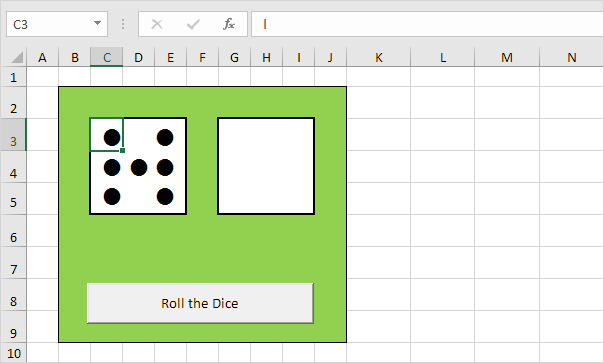
1. At the moment, each cell contains the letter l (as in lion). With a Wingdings font style, these l’s look like dots.

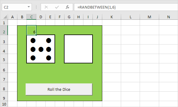
2. Enter the RANDBETWEEN function in cell C2.

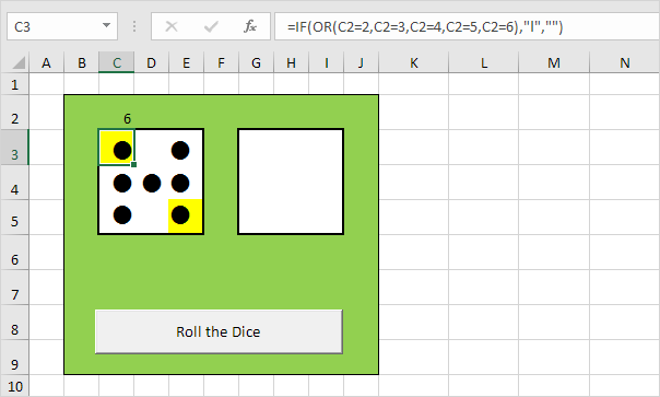
3. Enter the formula shown below into the yellow cells. If we roll 2, 3, 4, 5 or 6, these cells should contain a dot.

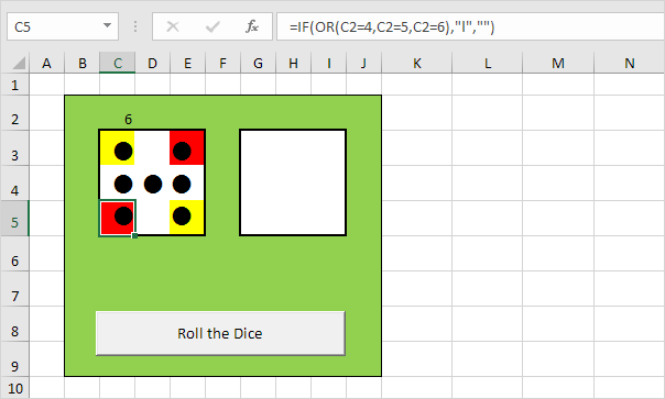
4. Enter the formula shown below into the red cells. If we roll 4, 5 or 6, these cells should contain a dot.

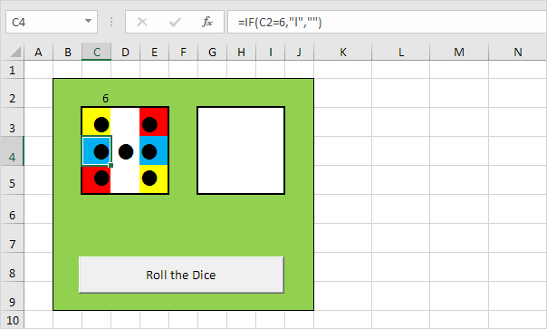
5. Enter the formula shown below into the blue cells. If we roll 6, these cells should contain a dot.

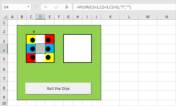
6. Enter the formula shown below into the gray cell. If we roll 1, 3 or 5, this cell should contain a dot.

7. Copy the range C2:E5 and paste it to the range G2:I5.

8. Change the font color of cell C2 and cell G2 to green (so the numbers are not visible).

9. Click the command button on the sheet (or press F9).

Result.