Nested IF function example in Excel
This tutorial shows how to calculate Nested IF function example in Excel using the example below;
Formula
=IF(T1,R1,IF(T2,R2,IF(T3,R3,IF(T4,R4,R5))))

Explanation
In the code above, T1-T5 represents 5 different logical tests, and R1-R5 represents 5 different results. You can see that each IF function requires it’s own set of parentheses.
This article describes the Excel nested IF construction. Usually, nested IFs are used when you need to test more than one condition and return different results depending on those tests.
Testing more than one condition
If you need to test for more than one condition, then take one of several actions, depending on the result of the tests, you can nest multiple IF statements together in one formula. You’ll often hear this referred to as “nested IFs”.
The idea of nesting comes from embedding or “nesting” one IF function inside another
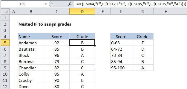
In the example shown, we are using nested IF functions to assign grades based on a score. The logic for assigning a grade goes like this:
| Score | Grade |
| 0-63 | F |
| 64-72 | D |
| 73-84 | C |
| 85-94 | B |
| 95-100 | A |
To build up a nested IF formula that reflects this logic, we can start by testing to see if the score is below 64. If TRUE, we return “F”. If FALSE, we move into the next IF function. This time, we test to see if the score is less than 73. If TRUE, we return “D”. If FALSE, we move into yet another IF function. And so on.
Eventually, the formula we have in cell D5 looks like this:
=IF(C5<64,"F",IF(C5<73,"D",IF(C5<85,"C",IF(C5<95,"B","A"))))
You can see that it’s important in this case to move in one direction, either low to high, or high to low. This allows us to return a result whenever a test returns TRUE, because we know that the previous tests have returned FALSE.
Making nested IFs easier to read
By their nature, nested IF formulas can be hard to read. If this bothers you, you can add line breaks inside the formula to “line up” the tests and results.