Example of COUNTIFS with variable table column in Excel

To use COUNTIFS with a variable table column, you can use INDEX and MATCH to find and retrieve the column for COUNTIFS. See example below:

Formula

=COUNTIFS(INDEX(Table,0,MATCH(name,Table[#Headers],0)),criteria))

Explanation

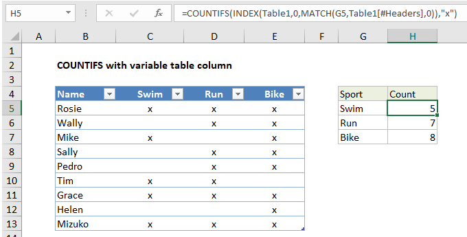
In the example shown, the formula in H5 is:

=COUNTIFS(INDEX(Table1,0,MATCH(G5,Table1[#Headers],0)),"x")

How this formula works

First, for context, it’s important to note that you can use COUNTIFS with a regular structured reference like this:

=COUNTIFS(Table1[Swim],"x")

This is a much simpler formula, but you can’t copy it down column H, because the column reference won’t change.

The example on this page therefore is meant to show one way to set up a formula that references a table with a variable column reference.

Working from the inside out, the MATCH function is used to find the position of the column name listed in column G:

MATCH(G5,Table1[#Headers],0)

MATCH uses the value in G5 as lookup value, the headers in Table1 for array, and 0 for match type to force an exact match. The result for G5 is 2, which goes into INDEX as the column number:

INDEX(Table1,0,2,0))

Notice row number has been set to zero, which causes INDEX to return the entire column, which is C5:C13 in this example.

This reference goes into COUNTIFS normally:

=COUNTIFS(C5:C13,"x")

COUNTIFS counts cells that contain “x”, and returns the result, 5 in this case.

When the formula is copied down column H, INDEX and MATCH return the correct column reference to COUNTIFS at each row.

Alternative with INDIRECT

The INDIRECT function can also be used to set up a variable column reference like this:

=COUNTIFS(INDIRECT("Table1["&G5&"]"),"x")

Note: INDIRECT is a volatile function and can cause performance problems in larger or more complicated workbooks.

Here, the structured reference is assembled as text, and INDIRECT evaluates the text as a proper cell reference.