Excel Data validation must begin with

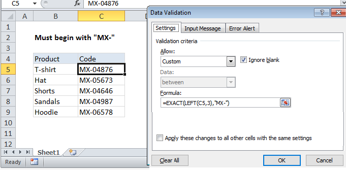
To allow only values that begin with certain text, you can use data validation with a custom formula based on the EXACT and LEFT functions.

In the example shown, the data validation applied to C5:C9 is:

=EXACT(LEFT(C5,3),"MX-")

How this formula works

Data validation rules are triggered when a user adds or changes a cell value.

In this formula, the LEFT function is used to extract the first 3 characters of the input in C5.

Next, the EXACT function is used to compare the extracted text to the text hard-coded into the formula, “MX-“.  EXACT performs a case-sensitive comparison. If the two text strings match exactly, EXACT returns TRUE and validation will pass. If the match fails, EXACT will return FALSE, and input will fail validation.

Non case-sensitive test with COUNTIF

If you don’t need a case-sensitive test, you can use a simpler formula based on the COUNTIF function with a wildcard:

=COUNTIF(C5,"MX-*")

The asterisk (*) is a wildcard that matches one or more characters.

Note: Cell references in data validation formulas are relative to the upper left cell in the range selected when the validation rule is defined, in this case C5.