Skip to content
Free Excel Tutorials
  • Home
  • Excel For Beginners
  • Excel Intermediate
  • Advanced Excel For Experts

Data Analysis

  • Everything about Charts in Excel
  • How to conditionally sum numeric data in an Excel table using SUMIFS
  • How to calculate correlation coefficient Correlation in Excel
  • Move chart to a separate worksheet in Excel
  • Error Bars in Excel

References

  • How to use Excel INDIRECT Function
  • Convert text string to valid reference in Excel using Indirect function
  • Two-way lookup with VLOOKUP in Excel
  • How to calculate two-way lookup VLOOKUP in Excel Table
  • How to get last row in numeric data in Excel

Data Validations

  • Excel Data validation must begin with
  • Excel Data validation require unique number
  • Excel Data validation number multiple 100
  • Excel Data validation must contain specific text
  • Excel Data validation with conditional list

How to calculate present value of annuity in excel

by

To get the present value of an annuity, you can use the PV function.

Formula

=PV(rate,periods,payment,0,0)

In the example shown, the formula in C9 is:

=PV(C5,C6,C4,0,0)

Explanation

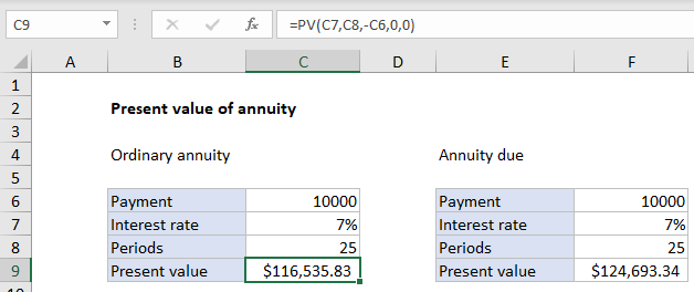
An annuity is a series of equal cash flows, spaced equally in time. In this example, an annuity pays 10,000 per year for the next 25 years, with an interest rate (discount rate) of 7%. To calculate present value, the PV function is configured as follows:

  • nper – the value from cell C8, 25.
  • pmt – the value from cell C6, 100000.
  • rate – the value from cell C7, 7%.
  • fv – 0.
  • type – 0, payment at end of period (regular annuity).

With this information, the present value of the annuity is $116,535.83. Note payment is entered as a negative number, so the result is positive.

Annuity due

With an annuity due, payments are made at the beginning of the period, instead of the end. To calculate present value for an annuity due, use 1 for the type argument. In the example shown, the formula in F9 is:

=PV(F7,F8,-F6,0,1)

Note the inputs (which come from column F) are the same as the original formula. The only difference is type = 1.

Post navigation

Previous Post:

DECIMAL function: Description, Usage, Syntax, Examples and Explanation

Next Post:

AVERAGE function: Description, Usage, Syntax, Examples and Explanation

Leave a Reply Cancel reply

Your email address will not be published. Required fields are marked *

Learn Basic Excel

Ribbon
Workbook
Worksheets
Format Cells
Find & Select
Sort & Filter
Templates
Print
Share
Protect
Keyboard Shortcuts

Categories

  • Charts
  • Data Analysis
  • Data Validation
  • Excel Functions
    • Cube Functions
    • Database Functions
    • Date and Time Functions
    • Engineering Functions
    • Financial Functions
    • Information Functions
    • Logical Functions
    • Lookup and Reference Functions
    • Math and Trig Functions
    • Statistical Functions
    • Text Functions
    • Web Functions
  • Excel VBA
  • Excel Video Tutorials
  • Formatting
  • Grouping
  • Others

Logical Functions

  • Return blank if in Excel
  • Check multiple cells are equal in Excel
  • How to use Excel XOR Function
  • How to use Excel OR Function
  • How to use Excel FALSE Function

Date Time

  • How to determine year is a leap year in Excel
  • Get first day of previous month in Excel
  • Steps to create Dynamic calendar grid in Excel
  • Convert date to text in Excel
  • Get project midpoint in Excel

Grouping

  • Map inputs to arbitrary values in Excel
  • If cell contains one of many things in Excel
  • Map text to numbers in Excel
  • Running count group by n size in Excel
  • Categorize text with keywords in Excel

General

  • 3D SUMIF for multiple worksheets in Excel
  • Hide and Unhide Columns or Rows in Excel
  • How to calculate percent variance in Excel
  • Excel Default Templates
  • List sheet names with formula in Excel
© 2026 xlsoffice . All Right Reserved. | Teal Smiles | Abbreviations And Their Meaning