Skip to content
Free Excel Tutorials
  • Home
  • Excel For Beginners
  • Excel Intermediate
  • Advanced Excel For Experts

Data Analysis

  • Working With Tables in Excel
  • Number and Text Filters Examples in Excel
  • How to count table rows in Excel
  • How To Perform and Interpret Regression Analysis in Excel
  • How to do a t-Test in Excel?

References

  • Left Lookup in Excel
  • Complete List of Excel Lookup and Reference Functions, References and Examples
  • Find closest match in Excel
  • Extract data with helper column in Excel
  • Extract all partial matches in Excel

Data Validations

  • Excel Data validation allow uppercase only
  • Excel Data validation whole percentage only
  • Data validation must not exist in list
  • Excel Data validation must not contain
  • Excel Data validation only dates between

Transpose: Switch ‘Rows to Columns’ or ‘Columns to Rows’ in Excel

by
  • Paste Special Transpose
  • Transpose Function

Use the ‘Paste Special Transpose’ option to switch rows to columns or columns to rows in Excel. You can also use the TRANSPOSE function.

Paste Special Transpose

To transpose data, execute the following steps.

Worked Example:   Cell References: Relative, Absolute and Mixed Referencing Examples

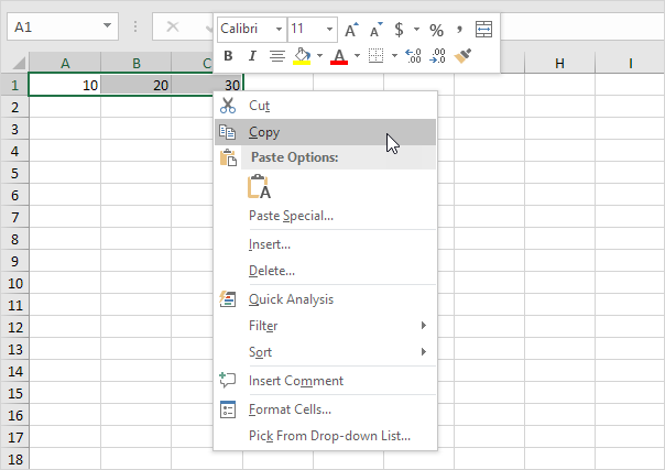
1. Select the range A1:C1.

2. Right click, and then click Copy.

3. Select cell E2.

4. Right click, and then click Paste Special.

5. Check Transpose.

6. Click OK.

Transpose Function

Also, TRANSPOSE function returns a vertical range of cells as a horizontal range, or vice versa.

To insert the TRANSPOSE function, execute the following steps.

Worked Example:   Sum Largest Numbers using LARGE function in Excel

1. First, select the new range of cells.

2. Type in =TRANSPOSE(

3. Select the range A1:C1 and close with a parenthesis.

Worked Example:   How to calculate percentage of total in Excel

4. Finish by pressing CTRL + SHIFT + ENTER.

Note: The formula bar indicates that this is an array formula by enclosing it in curly braces {}. To delete this array formula, select the range E2:E4 and press Delete.

Post navigation

Previous Post:

Lock Cells in a Worksheet Excel

Next Post:

How to use Union and Intersect operators in Excel

Leave a Reply Cancel reply

Your email address will not be published. Required fields are marked *

Learn Basic Excel

Ribbon
Workbook
Worksheets
Format Cells
Find & Select
Sort & Filter
Templates
Print
Share
Protect
Keyboard Shortcuts

Categories

  • Charts
  • Data Analysis
  • Data Validation
  • Excel Functions
    • Cube Functions
    • Database Functions
    • Date and Time Functions
    • Engineering Functions
    • Financial Functions
    • Information Functions
    • Logical Functions
    • Lookup and Reference Functions
    • Math and Trig Functions
    • Statistical Functions
    • Text Functions
    • Web Functions
  • Excel VBA
  • Excel Video Tutorials
  • Formatting
  • Grouping
  • Others

Logical Functions

  • Complete List of Excel Logical Functions, References and Examples
  • OR function: Description, Usage, Syntax, Examples and Explanation
  • Check multiple cells are equal in Excel
  • How to use Excel XOR Function
  • TRUE function: Description, Usage, Syntax, Examples and Explanation

Date Time

  • Add workdays no weekends in Excel
  • Display the current date in Excel
  • Get age from birthday in Excel
  • How to Calculate Age in Excel
  • Get days, hours, and minutes between dates in Excel

Grouping

  • Map text to numbers in Excel
  • Group times into 3 hour buckets in Excel
  • Categorize text with keywords in Excel
  • Group numbers at uneven intervals in Excel
  • Group times into unequal buckets in Excel

General

  • Mark Workbook as Final in Excel
  • Creating and Opening an existing file in Excel
  • Subtotal invoices by age in Excel
  • Excel Autofill Cell Ranges, Copy, Paste
  • Delete Blank Rows at Once in Excel
© 2023 xlsoffice . All Right Reserved. | Teal Smiles | Abbreviations And Their Meaning