
How to Use Solver Tool in Excel
Excel includes a tool called solver that uses techniques from the operations research to find optimal solutions for all kind of decision problems.
Load the Solver Add-in
To load the solver add-in, execute the following steps.
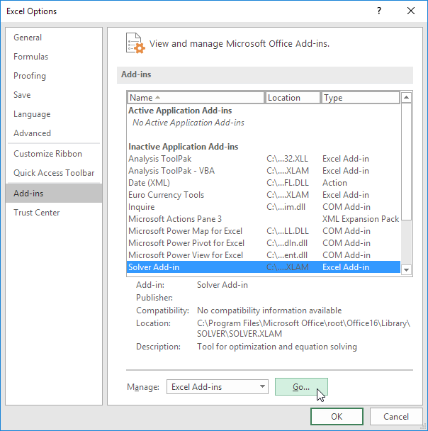
1. On the File tab, click Options.
2. Under Add-ins, select Solver Add-in and click on the Go button.
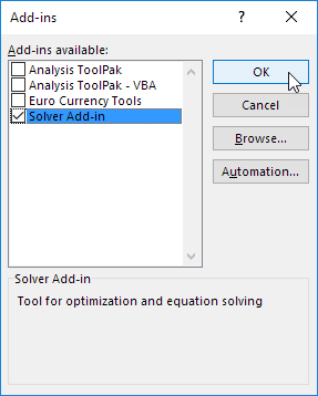
3. Check Solver Add-in and click OK.
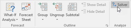
4. You can find the Solver on the Data tab, in the Analyze group.
Formulate the Model
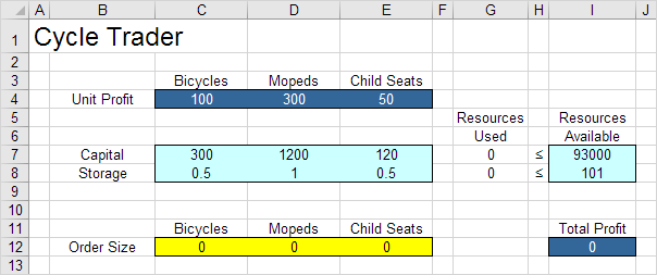
The model we are going to solve looks as follows in Excel.
1. To formulate this linear programming model, answer the following three questions.
a. What are the decisions to be made? For this problem, we need Excel to find out how much to order of each product (bicycles, mopeds and child seats).
b. What are the constraints on these decisions? The constrains here are that the amount of capital and storage used by the products cannot exceed the limited amount of capital and storage (resources) available. For example, each bicycle uses 300 units of capital and 0.5 unit of storage.
c. What is the overall measure of performance for these decisions? The overall measure of performance is the total profit of the three products, so the objective is to maximize this quantity.
2. To make the model easier to understand, name the following ranges.
| Range Name | Cells |
|---|---|
| UnitProfit | C4:E4 |
| OrderSize | C12:E12 |
| ResourcesUsed | G7:G8 |
| ResourcesAvailable | I7:I8 |
| TotalProfit | I12 |
3. Insert the following three SUMPRODUCT functions.
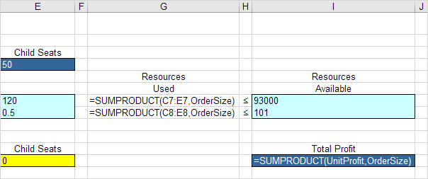
Explanation: The amount of capital used equals the sumproduct of the range C7:E7 and OrderSize. The amount of storage used equals the sumproduct of the range C8:E8 and OrderSize. Total Profit equals the sumproduct of UnitProfit and OrderSize.
Trial and Error
With this formulation, it becomes easy to analyze any trial solution.
For example, if we order 20 bicycles, 40 mopeds and 100 child seats, the total amount of resources used does not exceed the amount of resources available. This solution has a total profit of 19000.

It is not necessary to use trial and error. We shall describe next how the Excel Solver can be used to quickly find the optimal solution.
Solve the Model
To find the optimal solution, execute the following steps.
1. On the Data tab, in the Analyze group, click Solver.
Enter the solver parameters (read on). The result should be consistent with the picture below.
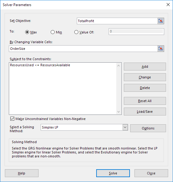
You have the choice of typing the range names or clicking on the cells in the spreadsheet.
2. Enter TotalProfit for the Objective.
3. Click Max.
4. Enter OrderSize for the Changing Variable Cells.
5. Click Add to enter the following constraint.

6. Check ‘Make Unconstrained Variables Non-Negative’ and select ‘Simplex LP’.
7. Finally, click Solve.
Result:
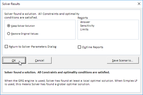
The optimal solution:
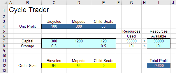
Conclusion: it is optimal to order 94 bicycles and 54 mopeds. This solution gives the maximum profit of 25600. This solution uses all the resources available.