Subtotal by color in Excel

This tutorial shows how to Subtotal by color in Excel using the example below;

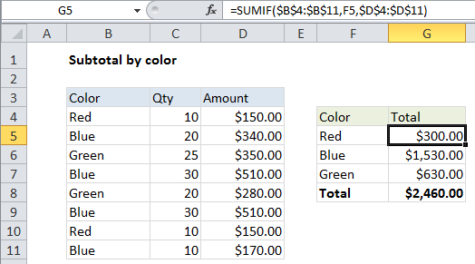
If you need to subtotal numbers by color, you can easily do so with the SUMIF function.

Formula

=SUMIF(color_range,criteria,number_range)

Explanation

In the example shown, the formula in G5 is:

=SUMIF($B$4:$B$11,F5,$D$4:$D$11)

How this formula works

The SUMIF function takes three arguments: range, criteria, and sum_range. In this case, we are using:

Range: $B$4:$B$11 – This is the set of cells to which the criteria (a color from column F in this case) will be applied. This is an absolute reference that won’t change when the formula is copied down.

Criteria: F5 – a relative address that will changed when copied down. This reference simply picks up the criteria from the adjacent cell in column F.

Sum_range: $D$4:$D$11 –  This is the set of cells being summed by SUMIF, when the supplied criteria is TRUE. This is an absolute reference that won’t change when the formula is copied down.

Note: if you’re looking for a way to count or sum cells filled with specific colors, it’s a more difficult problem. If you are using conditional formatting to apply colors, you can use the same logic to count or sum cells with formulas. If cells are filled with colors manually you’ll need a different approach.