Skip to content
xlsoffice. All Rights Reserved
  • Home
  • Excel For Beginners
  • Excel Intermediate
  • Advanced Excel For Experts

Lookup and Reference Examples

  • Find Closest Match in Excel Using INDEX, MATCH, ABS and MIN functions
  • How to use Excel COLUMN Function
  • Count rows that contain specific values in Excel
  • How to use Excel OFFSET function
  • Vlookup Examples in Excel

Data Analysis Examples

  • Managing Conditional Formatting Rules in Excel
  • How to create dynamic reference table name in Excel
  • Move chart to a separate worksheet in Excel
  • How to create Gauge Chart in Excel
  • How to combine 2 or more chart types in a single chart in Excel

Data Validation Examples

  • Excel Data validation no punctuation
  • Excel Data validation whole percentage only
  • Excel Data validation date in specific year
  • Excel Data validation allow weekday only
  • Excel Data validation number multiple 100

How to add Trendline to a chart in Excel

by

The essence of adding a trendline to chart  is to show visual data trends.

This example teaches you how to add a trendline to a chart in Excel.

1. Select the chart.

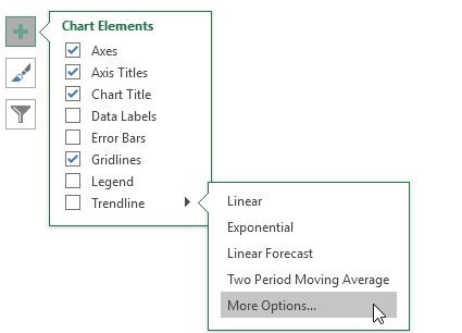
2. Click the + button on the right side of the chart, click the arrow next to Trendline and then click More Options.
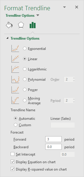
 The Format Trendline pane appears.

3. Choose a Trend/Regression type. Click Linear.

4. Specify the number of periods to include in the forecast. Type 3 in the Forward box.

5. Check “Display Equation on chart” and “Display R-squared value on chart”.
Result:
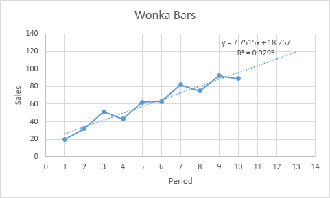
Explanation: Excel uses the method of least squares to find a line that best fits the points. The R-squared value equals 0.9295, which is a good fit. The closer to 1, the better the line fits the data. The trendline predicts 120 sold wonka bars in period 13. You can verify this by using the equation. y = 7.7515 * 13 + 18.267 = 119.0365.

Post navigation

Previous Post:

How To Create Budget in Excel

Next Post:

How to create Gauge Chart in Excel

Leave a Reply Cancel reply

Your email address will not be published. Required fields are marked *

Learn Basic Excel

Ribbon
Workbook
Worksheets
Format Cells
Find & Select
Sort & Filter
Templates
Print
Share
Protect
Keyboard Shortcuts

Categories

  • Charts
  • Data Analysis
  • Data Validation
  • Excel Functions
    • Cube Functions
    • Database Functions
    • Date and Time Functions
    • Engineering Functions
    • Financial Functions
    • Information Functions
    • Logical Functions
    • Lookup and Reference Functions
    • Math and Trig Functions
    • Statistical Functions
    • Text Functions
    • Web Functions
  • Excel VBA
  • Excel Video Tutorials
  • Formatting
  • Grouping
  • Others
  • Remove first character in a cell in Excel
  • UNICODE function: Description, Usage, Syntax, Examples and Explanation
  • How to translate letters to numbers in Excel
  • LEFT, LEFTB functions: Description, Usage, Syntax, Examples and Explanation
  • How to count line breaks in cell in Excel worksheet
  • Sum race time splits in Excel
  • Get date from day number in Excel
  • List holidays between two dates in Excel
  • Display the current date in Excel
  • HOUR function: Description, Usage, Syntax, Examples and Explanation
  • SYD function: Description, Usage, Syntax, Examples and Explanation
  • Example of Future value of annuity in Excel
  • SLN function: Description, Usage, Syntax, Examples and Explanation
  • PPMT function: Description, Usage, Syntax, Examples and Explanation
  • COUPNCD function: Description, Usage, Syntax, Examples and Explanation
© 2022 xlsoffice . All Right Reserved. | Teal Smiles