How to calculate next scheduled event in Excel

To get the next scheduled event from a list of events with dates, you can use an array formula based on the MIN and TODAY functions to find the next date, and INDEX and MATCH to display the event on that date.

Formula

{=MIN(IF((range>=TODAY()),range))}

Note: this is an array formula and must be entered with Control + Shift + Enter.

Explanation

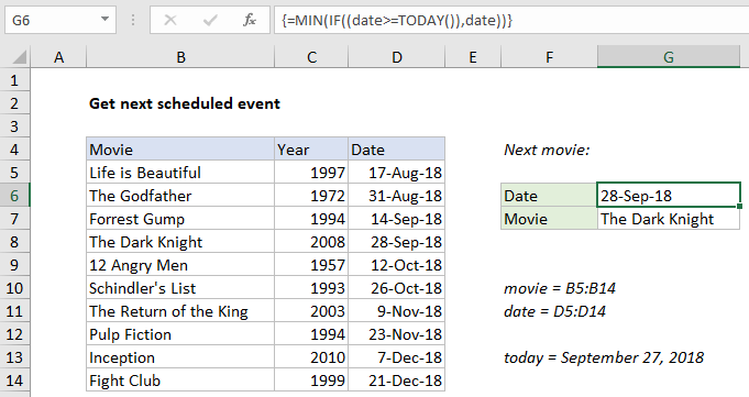
In the example shown, the formula in G6 is:

{=MIN(IF((date>=TODAY()),date))}

Where “date” is the named range D5:D14.

How this formula works

The first part of the solution uses the MIN and TODAY functions to find the “next date” based on the date today. This is done by filtering the dates through the IF function:

IF((date>=TODAY()),date)

The logical test generates an array of TRUE / FALSE values, where TRUE corresponds to dates greater than or equal to today:

{FALSE;FALSE;FALSE;TRUE;TRUE;TRUE;TRUE;TRUE;TRUE;TRUE}

When a result is TRUE, the date is passed into array returned by IF. When a result is FALSE, the date is replaced by the boolean FALSE. The IF function returns the following array to MIN:

{FALSE;FALSE;FALSE;43371;43385;43399;43413;43427;43441;43455}

The MIN function then ignores the FALSE values, and returns the smallest date value (43371), which is the date Sept. 28, 2018 in Excel’s date system.

Also See: Excel Advanced Lookup using Index and Match Functions

Getting the movie name

To display the movie associated with the “next date””, we use INDEX and MATCH:

=INDEX(movie,MATCH(G6,date,0))

Inside INDEX, MATCH finds the position of the date in G6 in the list of dates. This position, 4 in the example, is returned to INDEX as a row number:

=INDEX(movie,4)

and INDEX returns the movie at that position, “The Dark Knight”.

Also See: Highlight numbers that include symbols in Excel

All in one formula

To return the next Movie in a single formula, you can use this array formula:

{=INDEX(movie,MATCH(MIN(IF((date>=TODAY()),date)),date,0))}

With MINIFS

If you have a newer version of Excel, you can use the MINIFS function instead of the array formula in G6:

=MINIFS(date,date,">="&TODAY())

MINIFS was introduced in Excel 2016 via Office 365.

Handling errors

The formula on this page will work even when events aren’t sorted by date. However, if there are no upcoming dates, the MIN function will return zero instead of an error. This will display as the date “0-Jan-00” in G6, and the INDEX and MATCH formula will throw an #N/A error, since there is no zero-th row to get a value from. To trap this error, you can replace MIN with the SMALL function, then wrap the whole formula in IFERROR like this:

={IFERROR(SMALL(IF((date>=TODAY()),date),1),"None found")}

Unlike MIN, the SMALL function will throw an error when a value isn’t found, so IFERROR can be used to manage the error.

Also See: Minimum if multiple criteria in Excel