Calculate conditional mode with criteria in Excel

To calculate a conditional mode with one or more criteria you can use an array formula based on the IF and MODE functions.

Note: this is an array formula and must be entered with control + shift + enter.

Formula

{=MODE(IF(criteria,data))}

Explanation

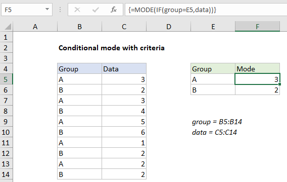
In the example shown, the formula in F5 is:

{=MODE(IF(group=E5,data))}

where “group” is the named range B5:B14, and “data” is the named range C5:C14.

How this formula works

The MODE function has no built-in way to apply criteria. If you give it a range, it will return the most frequently occurring number in the range.

To apply criteria, we use the IF function to test each data value in “group” to see if it matches the value in E5 (“A”):

IF(group=E5,data)

Because the logical test is based on an array containing multiple values (the named range “group”), the result is an array of TRUE FALSE results:

{TRUE;FALSE;TRUE;FALSE;TRUE;FALSE;TRUE;FALSE;TRUE;FALSE}

where each TRUE represents a row where the group is “A”. This array acts as a filter: for each TRUE, IF returns the corresponding value in the named range “data”. FALSE values remain unchanged. The final result of IF is this array:

{3;FALSE;3;FALSE;5;FALSE;1;FALSE;2;FALSE}

Notice only data values in group A have “survived”; group B values are now FALSE. This array goes into the MODE function, which returns the most frequently occurring number in group A, which is 3.

Note: when IF is used this way to filter values with an array operation, the formula must be entered with control + shift + enter.

Additional criteria

To apply more than one criteria, you can nest another IF inside the first IF:

{=MODE(IF(criteria1,IF(criteria2,data)))}