Examples of Sum with Or Criteria in Excel

How to sum data based upon multiple criteria?

Summing with Or criteria in Excel can be tricky. This article shows several easy to follow examples.

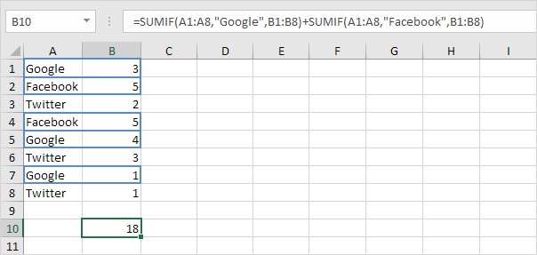
1. We start simple. For example, we want to sum the cells that meet the following criteria: Google or Facebook (one criteria range).

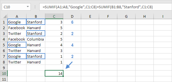
2a. However, if we want to sum the cells that meet the following criteria: Google or Stanford (two criteria ranges), we cannot simply use the  SUMIF  function twice (see the picture below). Cells that meet the criteria Google and Stanford are added twice, but they should only be added once. 10 is the answer we are looking for.

2b. We need an array formula. We use the IF function to check if Google or Stanford occurs.

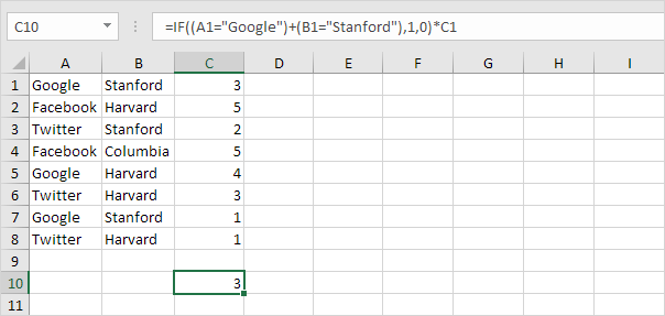
Explanation: TRUE = 1, FALSE = 0. For row 1, the IF function evaluates to IF(TRUE+TRUE,1,0)*3, IF(2,1,0)*3, 3. So the value 3 will be added. For row 2, the IF function evaluates to IF(FALSE+FALSE,1,0)*5, IF(0,1,0)*5, 0. So the value 5 will not be added. For row 3, the IF function evaluates to IF(FALSE+TRUE,1,0)*2, IF(1,1,0)*2, 2. So the value 2 will be added, etc.

2c. All we need is a SUM function that sums these values. To achieve this (don’t be overwhelmed), we add the SUM function and replace A1 with A1:A8, B1 with B1:B8 and C1 with C1:C8.

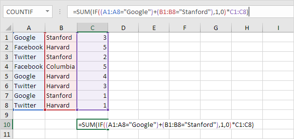
2d. Finish by pressing CTRL + SHIFT + ENTER.

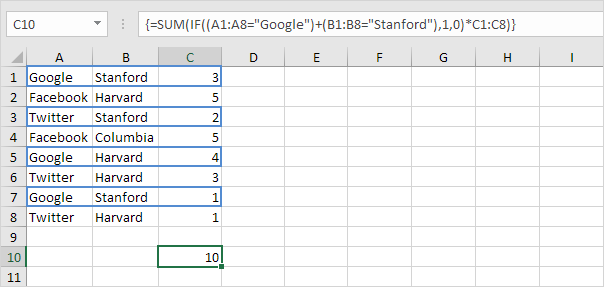
Note: The formula bar indicates that this is an array formula by enclosing it in curly braces {}. Do not type these yourself. They will disappear when you edit the formula.

Explanation: The range (array constant) created by the IF function is stored in Excel’s memory, not in a range. The array constant looks as follows:

{1;0;1;0;1;0;1;0}

multiplied by C1:C8 this yields:

{3;0;2;0;4;0;1;0}

This latter array constant is used as an argument for the SUM function, giving a result of 10.

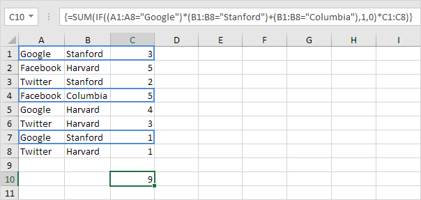
3. We can go one step further. For example, we want to sum the cells that meet the following criteria: (Google and Stanford) or Columbia.