Cell References: Relative, Absolute and Mixed Referencing Examples

Cell references in Excel are very important.

Building a structure or a template in excel using formula one needs to understand the difference between relative, absolute and mixed reference.

Relative Reference

To identify relative referencing, it is simply the ‘cell name’  as illustrated below.

N/B: Cell Name comprises of a column label and a row number of a selected cell.

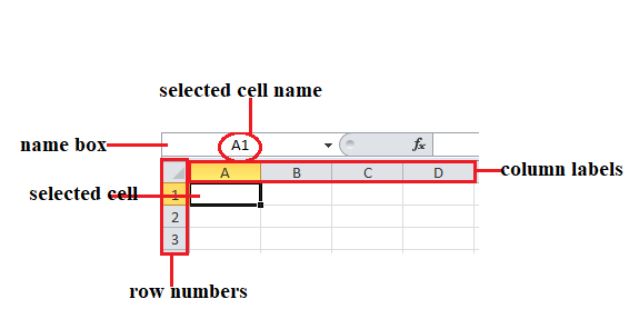
By default, Excel uses relative references. See the formula in cell D2 below. Cell D2 references (points to) cell B2 and cell C2. Both references are relative.

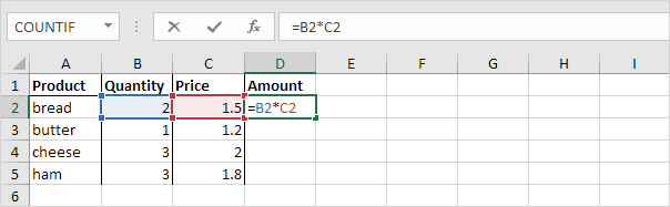
1. Select cell D2, click on the lower right corner of cell D2 and drag it down to cell D5.

Cell D3 references cell B3 and cell C3. Cell D4 references cell B4 and cell C4. Cell D5 references cell B5 and cell C5. In other words: each cell references its two neighbors on the left.

Absolute Reference

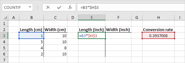
To identify absolute referencing, there is a dollar sign in front of the column label and a dollar sign in front of the row number, e.g $A$1.

See the formula in cell E3 below.

1. To create an absolute reference to cell H3, place a $ symbol in front of the column letter and row number ($H$3) in the formula of cell E3.

2. Now we can quickly drag this formula to the other cells.

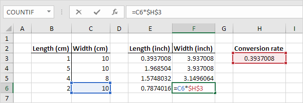
The reference to cell H3 is fixed (when we drag the formula down and across). As a result, the correct lengths and widths in inches are calculated.

Mixed Reference

Sometimes we need a combination of relative and absolute reference (mixed reference).

To identify Mixed Reference, there is a dollar sign either in front of the column label or in front of the row number, e.g $A1 or  A$1

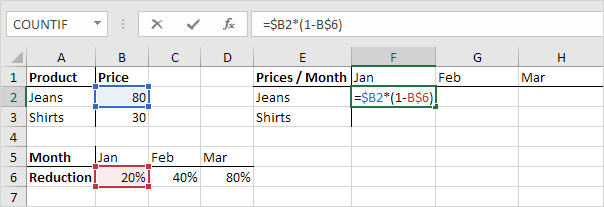
1. See the formula in cell F2 below.

2. We want to copy this formula to the other cells quickly. Drag cell F2 across one cell, and look at the formula in cell G2.

Do you see what happens? The reference to the price should be a fixed reference to column B. Solution: place a $ symbol in front of the column letter ($B2) in the formula of cell F2. In a similar way, when we drag cell F2 down, the reference to the reduction should be a fixed reference to row 6. Solution: place a $ symbol in front of the row number (B$6) in the formula of cell F2.

Result:

Note: we don’t place a $ symbol in front of the row number of $B2 (this way we allow the reference to change from $B2 (Jeans) to $B3 (Shirts) when we drag the formula down). In a similar way, we don’t place a $ symbol in front of the column letter of B$6 (this way we allow the reference to change from B$6 (Jan) to C$6 (Feb) and D$6 (Mar) when we drag the formula across).

3. Now we can quickly drag this formula to the other cells.

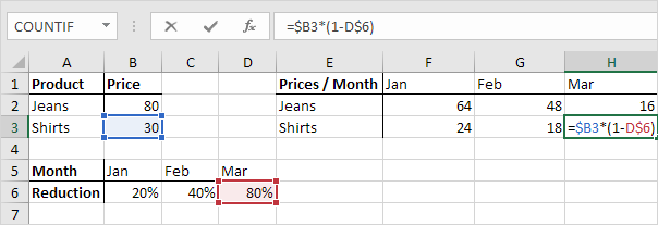
The references to column B and row 6 are fixed