Count if row meets internal criteria in Excel

This tutorial shows how to Count if row meets internal criteria in Excel using the example below;

To count rows in a table that meet internal, calculated criteria, without using a helper column, you can use the SUMPRODUCT function.

Formula

=SUMPRODUCT(--(logical_expression))

Explanation

Context

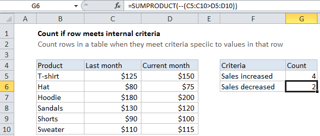
Imagine you have a table of sales figures for several products. You have a column for sales last month and a column for sales in the current month. You want to count products (rows) where current sales are less than sales last month. You can’t use COUNTIFs for this, because COUNTIFs is a range-based function. One option is to add a helper column that subtracts last month’s sales from this month’s sales, then use COUNTIF to count results less than zero. But what if you don’t want to (or can’t) add a helper column? In that case, you can can use SUMPRODUCT.

In the example shown, the formula in cell G6 is:

=SUMPRODUCT(--(C5:C10>D5:D10))

How this formula works

SUMPRODUCT is designed to work with arrays. It multiplies corresponding elements in two or more arrays and sums the resulting products. As a result, you can use SUMPRODUCT to process arrays that result from criteria being applied to a range of cells. The result of such operations will be arrays, which SUMPRODUCT can handle natively,  without requiring Control Shift Enter syntax.

In this case, we simply compare the values in column C to the values in column D using a logical expression:

C5:C10>D5:D10

Since we are dealing with ranges (arrays), the result is an array of TRUE FALSE values like this:

{FALSE;TRUE;FALSE;TRUE;FALSE;FALSE}

To coerce these into ones and zeros, we use a double negative operator (also called a double unary):

--(C5:C10>D5:D10)

Which produces and array like this:

{0;1;0;1;0;0}

which is then processed by SUMPRODUCT. Since there is only one array, SUMPRODUCT simply adds up the elements in the array and returns a total.