Count rows with at least n matching values

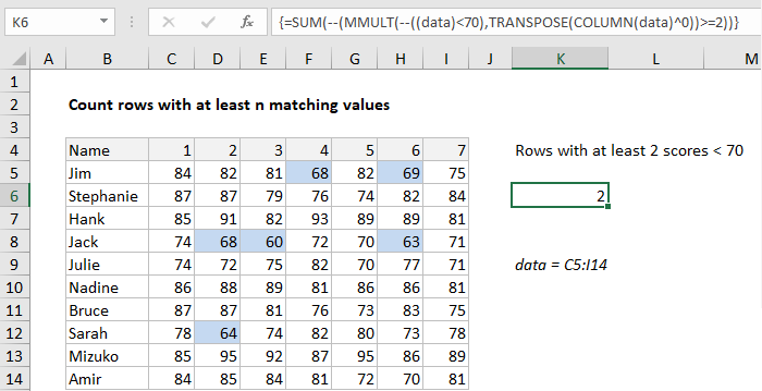
To count rows that contain specific values, you can use an array formula based on the MMULT, TRANSPOSE, COLUMN, and SUM functions. In the example shown, the formula in K6 is:

{=SUM(--(MMULT(--((data)<70),TRANSPOSE(COLUMN(data)^0))>=2))}

where data is the named range C5:I14.

Note this is an array formula and must be entered with control shift enter.

How this formula works

Working from the inside out, the logical criteria used in this formula is:

(data)<70

where data is the named range C5:I14. This generates a TRUE / FALSE result for every value in data, and the double negative coerces the TRUE FALSE values to 1 and 0 to yield an array like this:

{0,0,0,1,0,1,0;0,0,0,0,0,0,0;0,0,0,0,0,0,0;0,1,1,0,0,1,0;0,0,0,0,0,0,0;0,0,0,0,0,0,0;0,0,0,0,0,0,0;0,1,0,0,0,0,0;0,0,0,0,0,0,0;0,0,0,0,0,0,0}

Like the original data, this array is 10 rows by 7 columns (10 x 7) and goes into the MMULT function as array1. The next argument, array2 is created with:

TRANSPOSE(COLUMN(data)^0))

Here, the COLUMN function is used as a way to generate a numeric array of the right size, since matrix multiplication requires the column count in array1 (7) to equal the row count in array2.

The COLUMN function returns the 7-column array {3,4,5,6,7,8,9}. By raising this array to a power of zero, we end up with a 7 x 1 array like {1,1,1,1,1,1,1}, which TRANSPOSE changes to a 1 x 7 array like {1;1;1;1;1;1;1}.

MMULT then runs and returns a 10 x 1 array result {2;0;0;3;0;0;0;1;0;0}, which is processed with the logical expression >=2, resulting in an array of TRUE FALSE values:

{TRUE;FALSE;FALSE;TRUE;FALSE;FALSE;FALSE;FALSE;FALSE;FALSE}.

We again coerce TRUE FALSE to 1 and 0 with a double negative to get a final array inside SUM:

=SUM({1;0;0;1;0;0;0;0;0;0})

Which correctly returns 2, the number of names with at least 2 scores below 70.