Count unique text values with criteria

This tutorial shows how to Count unique text values with criteria using the example below;

Formula

{=SUM(--(FREQUENCY(IF(criteria,MATCH(values,values,0)),ROW(values)-ROW(valuesfirstcell)+1)>0))}

Explanation

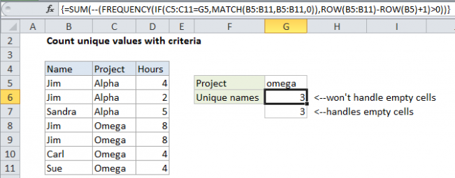
To count unique values in a range with a criteria, you can use an array formula based on the FREQUENCY function. Assume you have a list of employee names together with hours worked on “Project X”, and you want know how many employees worked on that  project. Looking at the data, you can see that the same employee names appear more than once, so what you want is a count of the unique names. In the example shown, the formula in G6 is:

{=SUM(--(FREQUENCY(IF(C5:C11=G5,MATCH(B5:B11,B5:B11,0)),ROW(B5:B11)-ROW(B5)+1)>0))}

Note: this is an array formula and must be entered with control + shift + enter.

How this formula works

This formula uses FREQUENCY to count unique numeric values that are derived with the MATCH function, which matches all values against themselves to determine a position.

Working from the inside, the MATCH function is used to get the position of each item that appears in the data. Because MATCH only returns the position of the “first match” values that appear more than once in the data return the same number.

Just outside of MATCH, the IF + criteria “filter” the values that MATCH works with so that it only returns MATCHES for rows that match criteria.

In the end, the array of positions generated by MATCH are fed to FREQUENCY in the data array argument.

The bins array argument is constructed from this part of the formula:

ROW(B3:B12)-ROW(B3)+1

which uses the row number of each item in the data and the row number of the first item in the data to build a straight, sequential array like this:

{1;2;3;4;5;6;7;8;9;10}

The FREQUENCY function returns an array of values that correspond to “bins”. In this case, we are supplying the same set of numbers for both the data array and bins array.

The result is that FREQUENCY returns an array of values that indicate the count that each value in the data array appears. This works because FREQUENCY is programmed to return zero for any numbers that appear more than once in the data array.

Next, each of these values is converted to TRUE or FALSE by the >0 construction, and then to 1 or zero with the double-unary (double-hyphen). This is done to force all non-zero values to 1.

Finally, SUMPRODUCT simply adds these values up and returns the total

Note: this is an array formula and must be entered using Control + Shift + Enter.

Handling empty cells in the range

If any of the cells in the range are empty, you’ll need to adjust the formula by adding an extra IF to prevent empty cells from being passed into the MATCH function, which will throw an error. The formula in G7 is:

{=SUM(--(FREQUENCY(IF(B5:B11<>"",IF(C5:C11=G5,MATCH(B5:B11,B5:B11,0))),ROW(B5:B11)-ROW(B5)+1)>0))}

With two criteria

If you have two criteria, you can extend the logic of the formula by adding another nested IF:

=SUM(--(FREQUENCY(IF(c1,IF(c2,MATCH(vals,vals,0))),ROW(vals)-ROW(vals.1st)+1)>0))

Where c1 = criteria1, c2 = criteria2 and vals = the values range.

With boolean logic

With boolean logic, you can reduce nested IFs:

=SUM(--(FREQUENCY(IF((criteria1)*(criteria2),MATCH(vals,vals,0)),ROW(vals)-ROW(vals.1st)+1)>0))

This makes it easier to add additional criteria.