Count cells that do not contain many strings in Excel

This tutorial shows how to Count cells that do not contain many strings in Excel using the example below;

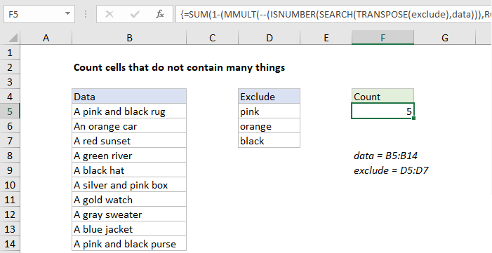
Formula

{=SUM(1-(MMULT(--(ISNUMBER(SEARCH(TRANSPOSE
(exclude),data))),ROW(exclude)^0)>0))}

Explanation

To count cells that do not contain many different strings, you can use a rather complex formula based on the MMULT function. In the example shown, the formula in F5 is:

{=SUM(1-(MMULT(--(ISNUMBER(SEARCH(TRANSPOSE
(exclude),data))),ROW(exclude)^0)>0))}

where “data” is the named range B5:B14, and “exclude” is the named range D5:D7.

Note: this is an array formula and must be entered with control + shift + enter

Comments

1. This formula is complicated considerably with the “contains” requirement. If you just need a formula to count cells that do not *equal* many things, you can use a more straightforward formula based on the MATCH function.
2. If you only have a limited number of strings to exclude, you can use the COUNTIFS function like this: =COUNTIFS(data,”<>*pink*”,data,”<>*orange*”,data,”<>*black*”). However, you’ll need to enter a new pair of range/criteria arguments for each string to exclude. In contrast, the formula explained below can handle a large number of strings to exclude entered directly on the worksheet.
3. This formula is complex. Let me know if you have a simpler formula to propose 🙂

How this formula works

The core of this formula is ISNUMBER and SEARCH:

ISNUMBER(SEARCH(TRANSPOSE(exclude),data))

Here, we transpose the items in the named range “exclude”, then feed the result to SEARCH as the “find text”, with data as “within text”. The SEARCH function returns a 2d array of TRUE and FALSE values, 10 rows by 3 columns, like this:

{3,#VALUE!,#VALUE!;#VALUE!,4,#VALUE!;#VALUE!,
#VALUE!,#VALUE!;#VALUE!,#VALUE!,#VALUE!;#VALUE!,#VALUE!,
3;#VALUE!,#VALUE!,#VALUE!;#VALUE!,#VALUE!,#VALUE!;
#VALUE!,#VALUE!,#VALUE!;#VALUE!,#VALUE!,
#VALUE!;#VALUE!,#VALUE!,#VALUE!}

For each value in “data”, we have 3 results (one per search string) that are either #VALUE errors or numbers. Numbers represent the position of a found text string, and errors represent text strings not found. By the way, the TRANSPOSE function is needed to generate the 10 x 3 array of complete results.

This array is fed into ISNUMBER to get TRUE FALSE values, which we convert to 1s and 0s with a double negative (–) operator. The result is an array like this:

{1,0,0;0,1,0;0,0,0;0,0,0;0,0,1;
0,0,0;0,0,0;0,0,0;0,0,0;0,0,0}

which goes into the MMULT function as array1. Following the rules of matrix multiplication, number of columns in array1 must equal the number of rows in array2. To generate array2, we use the ROW function like this:

ROW(exclude)^0

This yields an array of 1s, 3 rows by 1 column:

{1;1;1}

which goes into MMULT as array2. After array multiplication, we have an array dimensioned to match the original data:

{2;1;0;0;1;1;0;0;0;2}

In this array, any non-zero number represents a value where at least one of the excluded strings has been found. Zeros indicate no excluded strings were found. To force all non-zero values to 1, we use greater than zero:

{2;1;0;0;1;1;0;0;0;2}>0

which creates yet another array or TRUE and FALSE values:

{TRUE;TRUE;FALSE;FALSE;TRUE;
TRUE;FALSE;FALSE;FALSE;TRUE}

Our final goal is to count only text values where no excluded strings were found, so we need to reverse these values. Wo this by subtracting the array from 1. The math operation automatically coerces TRUE and FALSE values back to 1s and 0s, and we finally have an array to return to the SUM function:

=SUM({0;0;1;1;0;0;1;1;1;0})

The SUM function returns a final result of 5.