Skip to content
Free Excel Tutorials
  • Home
  • Excel For Beginners
  • Excel Intermediate
  • Advanced Excel For Experts

Data Analysis

  • How to add Trendline to a chart in Excel
  • How To Create Pareto Chart in Excel
  • How to Create Thermometer Chart in Excel
  • How to Use Solver Tool in Excel
  • How to Create Column Chart in Excel

References

  • How to get address of named range in Excel
  • How to get last row in text data in Excel
  • How to get address of last cell in range in Excel
  • How to get last row in mixed data with blanks in Excel
  • How to use Excel ROWS Function

Data Validations

  • Excel Data validation with conditional list
  • Excel Data validation don’t exceed total
  • Excel Data validation must contain specific text
  • Excel Data validation unique values only
  • How To Create Drop-down List in Excel

Check if range contains a value not in another range in Excel

by

To test if a range contains any values (i.e. at least one value) not in another range, you can use the SUMPRODUCT function with MATCH and ISNA.

The MATCH function receives a single lookup value, and returns a single match if any. In this case, however, we are giving MATCH an array for lookup value, so it will return an array of results, one per element in the lookup array.

See example below:

Formula

=SUMPRODUCT(--(ISNA(MATCH(rngA,rngB,0))))>0

Explanation

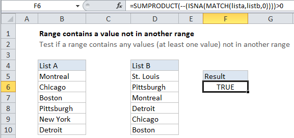
In the example shown, the formula in F6 is:

=SUMPRODUCT(--(ISNA(MATCH(lista,listb,0))))>0

How the formula works

MATCH is configured for “exact match”. If a match isn’t found, MATCH will return the #N/A error. After match runs, it returns have something like this:

=SUMPRODUCT(--(ISNA({3;5;6;2;#N/A;4})))>0

We take advantage of this by using the ISNA function to test for any #N/A errors.

After ISNA, we have:

=SUMPRODUCT(--({FALSE;FALSE;FALSE;FALSE;TRUE;FALSE}))>0

We use the double negative (double unary) operator to convert TRUE FALSE values to ones and zeros, which gives us this:

=SUMPRODUCT({0;0;0;0;1;0})>0

SUMPRODUCT then sums the elements in the array, and the result is compared to zero for force a TRUE or FALSE result.


Post navigation

Previous Post:

How to calculate project complete percentage in Excel

Next Post:

Popularly Used Excel Functions and their examples

Leave a Reply Cancel reply

Your email address will not be published. Required fields are marked *

Learn Basic Excel

Ribbon
Workbook
Worksheets
Format Cells
Find & Select
Sort & Filter
Templates
Print
Share
Protect
Keyboard Shortcuts

Categories

  • Charts
  • Data Analysis
  • Data Validation
  • Excel Functions
    • Cube Functions
    • Database Functions
    • Date and Time Functions
    • Engineering Functions
    • Financial Functions
    • Information Functions
    • Logical Functions
    • Lookup and Reference Functions
    • Math and Trig Functions
    • Statistical Functions
    • Text Functions
    • Web Functions
  • Excel VBA
  • Excel Video Tutorials
  • Formatting
  • Grouping
  • Others

Logical Functions

  • IF with boolean logic in Excel
  • OR function Examples in Excel
  • Check multiple cells are equal in Excel
  • How to use Excel AND Function
  • Return blank if in Excel

Date Time

  • Calculate years between dates in Excel
  • Two ways to sum time over 30 minutes in Excel
  • DATEVALUE function: Description, Usage, Syntax, Examples and Explanation
  • Convert text date dd/mm/yy to mm/dd/yy in Excel
  • Dynamic date list in Excel

Grouping

  • How to randomly assign data to groups in Excel
  • Categorize text with keywords in Excel
  • Map inputs to arbitrary values in Excel
  • Group times into 3 hour buckets in Excel
  • Group times into unequal buckets in Excel

General

  • How to create dynamic named range with INDEX in Excel
  • Basic text sort formula in Excel
  • How to calculate percent sold in Excel
  • Spell Check in Excel
  • Index and match on multiple columns in Excel
© 2026 xlsoffice . All Right Reserved. | Teal Smiles | Abbreviations And Their Meaning