Remove unwanted characters in Excel

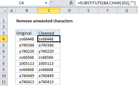
In the example shown, the formula in C4 is:

=SUBSTITUTE(B4,CHAR(202),"")

Which removes a series of 4 invisible characters at the start of each cell in column B.

How this formula works

The SUBSTITUTE function can find and replace text in a cell, wherever it occurs.

In this case, we are using SUBSTITUTE to find a character with code number 202, and replace it with an empty string (“”), which effectively removes the character completely.

How did I know to remove character 202?

To figure that out, I first used this formula to get the code number for the first character of B4:

=CODE(LEFT(B4))

Here, the LEFT function, without the optional second argument, returns the first character on the left. This goes into the CODE function, which reports the characters code value, which is 202.

All in one formula

In this case, since we are stripping leading characters, we could combine both formulas in one, like so:

=SUBSTITUTE(B4,CHAR(CODE(LEFT(B4))),"")

Here, instead of providing character 202 explicitly to SUBSTITUTE, we are using CODE and CHAR to provide a code dynamically, using the first character in the cell.