Count matches between two columns in Excel

This tutorial shows how to Count matches between two columns in Excel using the example below;

Formula

=SUMPRODUCT(--(range1=range2))

Explanation

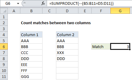
If you want to compare two columns and count matches in corresponding rows, you can use the SUMPRODUCT function with a simple comparison of the two ranges. For example, if you have values in B5:B11 and C5:C11 and you want to count any differences, you can use this formula:

=SUMPRODUCT(--(B5:B11=C5:C11))

How this formula works

The SUMPRODUCT function is a versatile function that handles arrays natively without any special array syntax. Its behavior is simple: it multiplies, then sums the product of arrays. In the example shown, the expression B5:B11 = C5:C11 will generate an array that contains TRUE and FALSE values like this:

{TRUE;TRUE;FALSE;TRUE;FALSE;FALSE;FALSE}

Note that we have 3 TRUE values because there are 3 matches.

In this state, SUMPRODUCT will actually return zero because TRUE and FALSE values are not counted as numbers in Excel by default. To get SUMPRODUCT to treat TRUE as 1 and FALSE as zero, we need to “coerce” them into numbers. The double negative is a simple way to do that:

--(B5:B11=C5:C11)

After coercion, we have:

{1;1;0;1;0;0;0}

With no other arrays to multiply, SUMPRODUCT simply sums the values and returns 3.

Count non-matching rows

To count non-matching values, you can reverse the logic like so:

=SUMPRODUCT(--(B5:B11<>C5:C11))