How to use IFS function in Excel

Use the IFS function in Excel 2016 when you have multiple conditions to meet. The IFS function returns a value corresponding to the first TRUE condition.

Note: if you don’t have Excel 2016, you can nest the IF function.

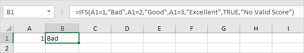
1a. If the value in cell A1 equals 1, the IFS function returns Bad.

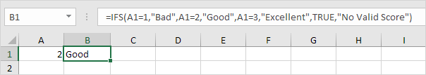
1b. If the value in cell A1 equals 2, the IFS function returns Good.

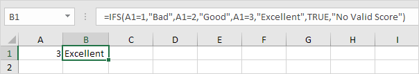
1c. If the value in cell A1 equals 3, the IFS function returns Excellent.

1d. If the value in cell A1 equals another value, the IFS function returns No Valid Score.

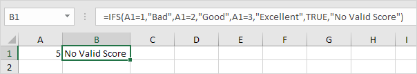
Note: instead of TRUE, you can also use 1=1 or something else that is always TRUE.

Here’s another example.

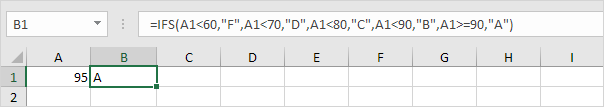
2a. If the value in cell A1 is less than 60, the IFS function returns F.

2b. If the value in cell A1 is greater than or equal to 60 and less than 70, the IFS function returns D.

2c. If the value in cell A1 is greater than or equal to 70 and less than 80, the IFS function returns C.

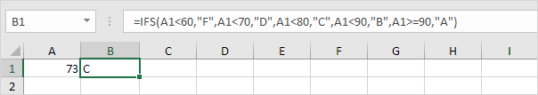
2d. If the value in cell A1 is greater than or equal to 80 and less than 90, the IFS function returns B.

2e. If the value in cell A1 is greater than or equal to 90, the IFS function returns A.

Note: to slightly change the boundaries, you might want to use “<=” instead of “<” in your own function.