Count rows that contain specific values in Excel

This tutorial shows how to Count rows that contain specific values in Excel using the example below;

Formula

=SUM(--(MMULT(--(criteria),TRANSPOSE(COLUMN(data)))>0))

Explanation

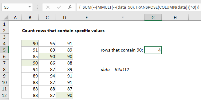
To count rows that contain specific values, you can use an array formula based on the MMULT, TRANSPOSE, COLUMN, and SUM functions. In the example shown, the formula in G5 is:

{=SUM(--(MMULT(--(data=90),TRANSPOSE(COLUMN(data)))>0))}

where data is the named range B4:B12.

Note: this is an array formula and must be entered with control shift enter.

How this formula works

Working from the inside out, the logical criteria used in this formula is:

--(data=90)

where data is the named range B4:D12. This generates a TRUE / FALSE result for every value in data, and the double negative coerces the TRUE FALSE values to 1 and 0 to yield an array like this:

{1,0,0;0,0,0;0,1,1;1,0,0;0,0,0;0,0,0;0,0,0;0,0,0;0,0,1}

Like the original data, this array is 9 rows by 3 columns (9 x 3) and goes into the MMULT function as array1.

Array2 is derived with:

TRANSPOSE(COLUMN(data))

This is the tricky and fun part of this formula. The COLUMN function is used simply for convenience as a way to generate a numeric array of the right size. To perform matrix multiplication with MMULT, the column count in array1 (3) must equal the row count in array2.

COLUMN returns the 3-column array {2,3,4}, and TRANSPOSE changes this array to the the 3-row array {2;3;4}. MMULT then runs and returns a 9 x 1 array result:

=SUM(--({2;0;7;2;0;0;0;0;4}>0))

We check for non-zero entries with >0 and again coerce TRUE FALSE to 1 and 0 with a double negative to get a final array inside SUM:

=SUM({1;0;1;1;0;0;0;0;1})

In this final array, a 1 represents a row where the logical test (data=90) returned true. The total returned by SUM is a count of all rows that contain the number 90.

Literal contains

If you need to check for specific text values, in other words, literally check to see if cells contain certain text values, you can change the logic in the formula on this page to use the ISNUMBER and SEARCH function. For example, to count cells/rows that contain “apple” you can use:

=ISNUMBER(SEARCH("apple",data))