Skip to content
xlsoffice. All Rights Reserved
  • Home
  • Excel For Beginners
  • Excel Intermediate
  • Advanced Excel For Experts

Lookup and Reference Examples

  • Vlookup Examples in Excel
  • How to get last row in numeric data in Excel
  • How to use Excel MMULT Function
  • Approximate match with multiple criteria in Excel
  • How to get address of first cell in range in Excel

Data Analysis Examples

  • Calculate Conditional Percentile ‘IF’ in table in Excel
  • How to calculate correlation coefficient Correlation in Excel
  • How to sum a total in multiple Excel tables
  • Managing Conditional Formatting Rules in Excel
  • Randomize/ Shuffle List in Excel

Data Validation Examples

  • Excel Data validation whole percentage only
  • How To Create Drop-down List in Excel
  • Excel Data validation don’t exceed total
  • Data validation must not exist in list
  • Prevent invalid data entering in specific cells

How To Create Pareto Chart in Excel

by

This chapter teaches you how to create a Pareto Chart in Excel. The Pareto principle states that, for many events, roughly 80% of the effects come from 20% of the causes. In this example, we will see that roughly 80% of the complaints come from 20% of the complaint types.

To create a Pareto chart in Excel 2016, execute the following steps.

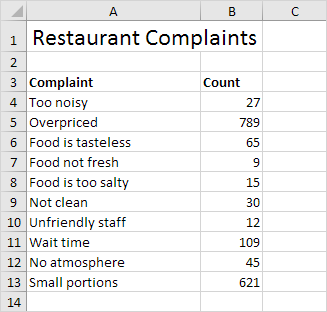
1. Select the range A3:B13.

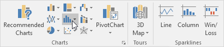
2. On the Insert tab, in the Charts group, click the Histogram symbol.
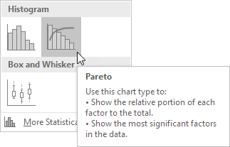
3. Click Pareto.

Result:

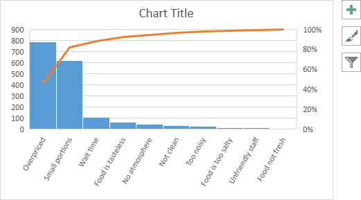
Note: a Pareto chart combines a column chart and a line graph.

4. Enter a chart title.

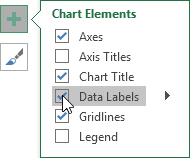
5. Click the + button on the right side of the chart and click the check box next to Data Labels.

Result:

Conclusion: the orange Pareto line shows that (789 + 621) / 1722 ≈ 80% of the complaints come from 2 out of 10 = 20% of the complaint types (Overpriced and Small portions). In other words: the Pareto principle applies

Post navigation

Previous Post:

Everything about Charts in Excel

Next Post:

Convert Negative Numbers to Zero in Excel

Leave a Reply Cancel reply

Your email address will not be published. Required fields are marked *

Learn Basic Excel

Ribbon
Workbook
Worksheets
Format Cells
Find & Select
Sort & Filter
Templates
Print
Share
Protect
Keyboard Shortcuts

Categories

  • Charts
  • Data Analysis
  • Data Validation
  • Excel Functions
    • Cube Functions
    • Database Functions
    • Date and Time Functions
    • Engineering Functions
    • Financial Functions
    • Information Functions
    • Logical Functions
    • Lookup and Reference Functions
    • Math and Trig Functions
    • Statistical Functions
    • Text Functions
    • Web Functions
  • Excel VBA
  • Excel Video Tutorials
  • Formatting
  • Grouping
  • Others
  • How to pad text to match equal length in Excel
  • Replace one character with another in Excel
  • LEFT, LEFTB functions: Description, Usage, Syntax, Examples and Explanation
  • How to use double quotes inside a formula in Excel
  • How to count keywords in a range of cell
  • How to calculate next day of week in Excel
  • Add months to date in Excel
  • Count holidays between two dates in Excel
  • Get project end date in Excel
  • ISOWEEKNUM function: Description, Usage, Syntax, Examples and Explanation
  • YIELDMAT function: Description, Usage, Syntax, Examples and Explanation
  • EFFECT function: Description, Usage, Syntax, Examples and Explanation
  • IRR function: Description, Usage, Syntax, Examples and Explanation
  • How to calculate compound interest in Excel
  • ODDFPRICE function: Description, Usage, Syntax, Examples and Explanation
Acronyms, Abbreviations, Initialism & What They Stand For
© 2022 xlsoffice . All Right Reserved. | Teal Smiles