3D SUMIF for multiple worksheets in Excel

This tutorial shows how to 3D SUMIF for multiple worksheets in Excel using the example below;

Formula

=SUMPRODUCT(SUMIF(INDIRECT
("'"&sheets&"'!"&"range"),criteria,
INDIRECT("'"&sheets&"'!"&"sumrange")))

Explanation

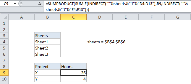
To conditionally sum identical ranges that exist in separate worksheets, all in one formula, you can do so with the SUMIF function + INDIRECT, wrapped in SUMPRODUCT. In the example, the formula looks like this:

=SUMPRODUCT(SUMIF(INDIRECT
("'"&sheets&"'!"&"D4:D5"),B9,
INDIRECT("'"&sheets&"'!"&"E4:E5")))

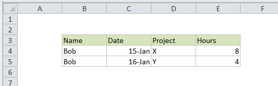
The data on each of the three sheets being processed looks like this:

Explanation

First of all, note that you can’t use SUMIFs with a “normal” 3D reference like this:

Sheet1:Sheet3!D4:D5
This is the standard “3D syntax” but if you try to use it with SUMIF, you’ll get a #VALUE error. So, to workaround this problem you can use a named range “sheets” that lists each sheet (worksheet tab) that you want to include. However, to build references that Excel will interpret correctly, we need to concatenate the sheet names to the ranges we need to work with and then use the INDIRECT to get Excel to recognize them correctly.

Also, because the named range “sheets” contains multiple values (i.e. its an array), the result of SUMIF in this case is also an array (sometimes called a “resultant array). So, we use SUMPRODUCT to handle it, since SUMPRODUCT has the ability to handle arrays natively without requiring Ctrl-Shift-Enter, like many other array formulas.

Alternatively;

The example above is somewhat complicated. Another way to handle this problem is to do a “local” conditional sum on each sheet, then use a regular 3D sum to add up each value on the summary tab.

To do this, add a SUMIF formula to each sheet sheet that uses a criteria cell on the summary sheet. Then when you change the criteria, all linked SUMIF formulas will update.