Round a number down to nearest multiple in Excel

This tutorials shows how to Round a number down to nearest multiple in Excel.

If you need to round a number down to the nearest specified multiple (i.e. round a number down to the nearest dollar, down to the nearest $.25, down to the nearest multiple of 5, etc.) you can use the FLOOR function.

Formula

=FLOOR(number,multiple)

Explanation

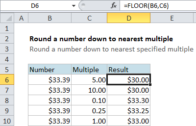
In the example, the formula in cell D6 is

=FLOOR(B6,C6)

This tells Excel to take the value in B6 ($33.39 ) and round it down to the nearest multiple of the value in C6 (5). The result is $30.00, since 30 is the multiple of 5 before 33.39. Likewise, in cell D7, we get 30 when rounding down using a multiple of 10.

You can use FLOOR to round prices, times, instrument readings or any other numeric value.

Note that FLOOR rounds down using the multiple supplied. You can use the MROUND function to round to the nearest multiple and the CEILING function to round up with a multiple.