
Skip to content
Free Excel Tutorials
  • Home
  • Excel For Beginners
  • Excel Intermediate
  • Advanced Excel For Experts

Data Analysis

  • Example of COUNTIFS with variable table column in Excel
  • How to create Checklist in Excel
  • Create Scatter Chart in Excel
  • How to calculate correlation coefficient Correlation in Excel
  • Conditional Formatting Rules in Excel

References

  • MATCH function: Description, Usage, Syntax, Examples and Explanation
  • Vlookup Examples in Excel
  • Lookup entire row in Excel
  • How to get address of named range in Excel
  • Find closest match in Excel

Data Validations

  • Excel Data validation specific characters only
  • Excel Data validation must begin with
  • Excel Data validation number multiple 100
  • Excel Data validation allow uppercase only
  • Excel Data validation date in specific year

Excel Rank if formula Example

by

This tutorials shows how to rank items in a list using one or more criteria in Excel.

To achieve this you can use the COUNTIFS function.

Formula

=COUNTIFS(criteria_range,criteria,values,">"&value)+1
Explanation

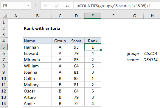
In the example shown, the formula in E5 is:

=COUNTIFS(groups,C5,scores,">"&D5)+1

where “groups” is the named range C5:C14, and “scores” is the named range D5:D14.

The result is a rank for each person in their own group. Note: although data is sorted by group in the screenshot, the formula will work fine with unsorted data.

How this formula works

Although Excel has a RANK function, there is no RANKIF function to perform a conditional rank. However, you can easily create a conditional RANK with the COUNTIFS function.

The COUNTIFS function can perform a conditional count using two or more criteria. Criteria are entered in range/criteria pairs. In this case, the first criteria restricts the count to the same group, using the named range “groups” (C5:C14):

=COUNTIFS(groups,C5)

By itself, this will return total group members in group “A”, which is 5.

The second criteria restricts the count to only scores greater than the “current score” from D5:

=COUNTIFS(groups,C5,scores,">"&D5)

The two criteria work together to count rows where the group is A and the score is higher. For the first name in the list (Hannah), there are no higher scores in group A, so COUNTIFS returns zero. In the next row (Edward), there are three scores in group A higher than 79, so COUNTIFS returns 3. And so on.

To get a proper rank, we simply add 1 to the number returned by COUNTIFS.

Reversing rank order

To reverse rank order and rank in order (i.e. smallest value is ranked #1) just use the less than operator (<) instead of greater than (>):

=COUNTIFS(groups,C5,scores,"<"&D5)+1

Instead of counting scores greater than D5, this version will count scores less than the value in D5, effectively reversing the rank order.

Post navigation

Previous Post:

DECIMAL function: Description, Usage, Syntax, Examples and Explanation

Next Post:

AVERAGE function: Description, Usage, Syntax, Examples and Explanation

Leave a Reply Cancel reply

Your email address will not be published. Required fields are marked *

Learn Basic Excel

Ribbon
Workbook
Worksheets
Format Cells
Find & Select
Sort & Filter
Templates
Print
Share
Protect
Keyboard Shortcuts

Categories

  • Charts
  • Data Analysis
  • Data Validation
  • Excel Functions
    • Cube Functions
    • Database Functions
    • Date and Time Functions
    • Engineering Functions
    • Financial Functions
    • Information Functions
    • Logical Functions
    • Lookup and Reference Functions
    • Math and Trig Functions
    • Statistical Functions
    • Text Functions
    • Web Functions
  • Excel VBA
  • Excel Video Tutorials
  • Formatting
  • Grouping
  • Others

Logical Functions

  • Nested IF function example in Excel
  • IF, AND, OR and NOT Functions Examples in Excel
  • Complete List of Excel Logical Functions, References and Examples
  • SWITCH function example in Excel
  • IFERROR function: Description, Usage, Syntax, Examples and Explanation

Date Time

  • Display the current date in Excel
  • Sum through n months in Excel
  • How to get workdays between dates in Excel
  • How to enter Today’s Date or Static Date and Time in Excel
  • Add days exclude certain days of week in Excel

Grouping

  • Group numbers with VLOOKUP in Excel
  • Group times into 3 hour buckets in Excel
  • How to randomly assign people to groups in Excel
  • If cell contains one of many things in Excel
  • Map inputs to arbitrary values in Excel

General

  • Transpose: Switch ‘Rows to Columns’ or ‘Columns to Rows’ in Excel
  • Common Errors in Excel
  • Create dynamic workbook reference to another workbook in Excel
  • How to choose page/paper size in Excel before Printing
  • How to calculate percentage of total in Excel
© 2026 xlsoffice . All Right Reserved. | Teal Smiles | Abbreviations And Their Meaning