Skip to content
xlsoffice. All Rights Reserved
  • Home
  • Excel For Beginners
  • Excel Intermediate
  • Advanced Excel For Experts

Lookup and Reference Examples

  • Merge tables with VLOOKUP in Excel
  • Two-column Lookup in Excel
  • Basic INDEX MATCH approximate in Excel
  • Multi-criteria lookup and transpose in Excel
  • How to get address of named range in Excel

Data Analysis Examples

  • How to sum a total in multiple Excel tables
  • Create Scatter Chart in Excel
  • How to count table columns in Excel
  • Conditional Formatting Icon Sets Examples in Excel
  • Conditional Formatting Color Scales Examples in Excel

Data Validation Examples

  • Excel Data validation allow weekday only
  • How To Create Drop-down List in Excel
  • Prevent invalid data entering in specific cells
  • Excel Data validation unique values only
  • Excel Data validation date in specific year

Lock Cells in a Worksheet Excel

by
  • Lock specific areas of a worksheet

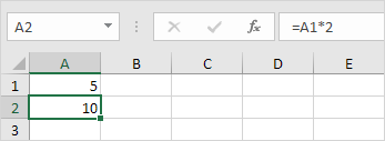
You can lock cells in Excel if you want to protect cells from being edited. In this example, we will lock cell A2.

Before you start: by default, all cells are locked. However, locking cells has no effect until you protect the worksheet. So when you protect a worksheet, all your cells (=worksheet) will be locked. As a result, if you want to lock a cell, you have to unlock all cells first, lock a cell, and then protect the sheet.

Worked Example:   Things you find in Excel Status Bar

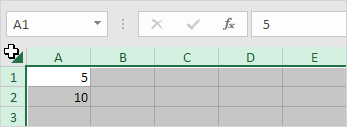
1. Select all cells.

Worked Example:   Freeze and Unfreeze Panes in Excel

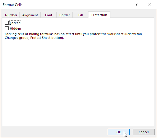
2. Right click, and then click Format Cells.

3. On the Protection tab, uncheck the Locked check box and click OK.

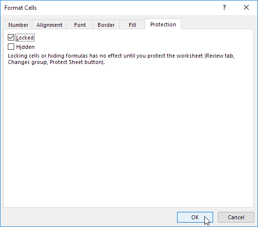
4. Right click cell A2, and then click Format Cells.

5. On the Protection tab, check the Locked check box and click OK.

Worked Example:   Password Protect Macro in Excel

Note: if you also check the Hidden check box, users cannot see the formula in the formula bar when they select cell A2.

6. Protect the sheet.

Cell A2 is locked now. To edit cell A2, you have to unprotect the sheet.

Post navigation

Previous Post:

How To Create Loan Amortization Schedule in Excel

Next Post:

RAND vs RANDBETWEEN function examples in Excel

Leave a Reply Cancel reply

Your email address will not be published. Required fields are marked *

Learn Basic Excel

Ribbon
Workbook
Worksheets
Format Cells
Find & Select
Sort & Filter
Templates
Print
Share
Protect
Keyboard Shortcuts

Categories

  • Charts
  • Data Analysis
  • Data Validation
  • Excel Functions
    • Cube Functions
    • Database Functions
    • Date and Time Functions
    • Engineering Functions
    • Financial Functions
    • Information Functions
    • Logical Functions
    • Lookup and Reference Functions
    • Math and Trig Functions
    • Statistical Functions
    • Text Functions
    • Web Functions
  • Excel VBA
  • Excel Video Tutorials
  • Formatting
  • Grouping
  • Others
  • Convert Numbers to Text in Excel
  • How to find nth occurrence of character in Excel
  • Excel MAX, MATCH and ADDRESS function illustration
  • RIGHT, RIGHTB functions: Description, Usage, Syntax, Examples and Explanation
  • LOWER function: Description, Usage, Syntax, Examples and Explanation
  • Display Days in month in Excel
  • NETWORKDAYS.INTL function: Description, Usage, Syntax, Examples and Explanation
  • Convert date string to date time in Excel
  • Convert decimal minutes to Excel time
  • How to calculate project start date based on end date in Excel
  • RRI function: Description, Usage, Syntax, Examples and Explanation
  • COUPNUM function: Description, Usage, Syntax, Examples and Explanation
  • RECEIVED function: Description, Usage, Syntax, Examples and Explanation
  • Example of Future value of annuity in Excel
  • PRICEMAT function: Description, Usage, Syntax, Examples and Explanation
© 2022 xlsoffice . All Right Reserved. | Teal Smiles