Count unique text values in a range in Excel
This tutorial shows how to Count unique text values in a range in Excel using the example below;
Formula
=SUMPRODUCT(--(FREQUENCY(MATCH(data,data,0),ROW(data)-ROW(data.firstcell)+1)>0))
Explanation
If you need to count unique text values in a range, you can use a formula that uses several functions: FREQUENCY , MATCH, ROW and SUMPRODUCT.
It’s also possible to use COUNTIF, as explained below.
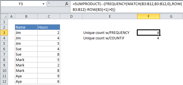
Assume you have a list of employee names together with hours worked on “Project X”, and you want know how many employees worked on that project. Looking at the data, you can see that the same employee names appear more than once, so what you want is a count of the unique names.
The employee names appear in the range B3:B12. To get a count of unique names, you can use the following formula:
=SUMPRODUCT(--(FREQUENCY(MATCH(B3:B12,B3:B12,0),ROW(B3:B12)-ROW(B3)+1)>0))
How this formula works
This formula is more complicated than a similar formula that uses FREQUENCY to count unique numeric values because FREQUENCY doesn’t work with non-numeric values. As a result, a large part of the formula simply transforms the non-numeric data into numeric data that FREQUENCY can handle.
Working from the inside, the MATCH function is used to get the position of each item that appears in the data. Because MATCH only returns the position of the “first match” values that appear more than once in the data return the same number.
Because MATCH receives an array of values for the match_value argument, it returns an array of positions. These are fed to FREQUENCY in the data array argument.
{1;1;1;4;4;6;6;6;9;9}
The bins array argument is constructed from this part of the formula:
ROW(B3:B12)-ROW(B3)+1
which uses the row number of each item in the data and the row number of the first item in the data to build a straight, sequential array like this:
{1;2;3;4;5;6;7;8;9;10}
The FREQUENCY function returns an array of values that correspond to “bins”. In this case, we supply the array returned by MATCH for the data array, and the array returned by ROW code above as the bins array.
The result is that FREQUENCY returns an array of values that indicate the count that each value in the data array appears. FREQUENCY has a special feature that automatically returns zero for any numbers that appear more than once in the data array, so the result array looks like this:
{3;0;0;2;0;3;0;0;2;0;0}
Next, each of these values is converted to TRUE or FALSE by the >0 construction, and then to 1 or zero with the double-unary (double-hyphen). This is done because SUMPRODUCT needs numeric values, it can’t work directly with text or logical values.
Inside the SUMPRODUCT function the final array looks like this:
{1;0;0;1;0;1;0;0;1;0;0}
Finally, SUMPRODUCT simply adds these values up and returns the total, which in this case is 4.
Handling empty cells in the range
If any of the cells in the range are empty, and you want to use FREQUENCY instead of COUNTIF, you’ll need use a more complicated array formula that includes IF:
{=SUM(IF(FREQUENCY(IF(data<>"", MATCH(data,data,0)),ROW(data)-ROW(data.firstcell)+1),1))}
Note: because the logical test portion of the IF statement contains an array, the formula becomes an array formula that requires Control-Shift-Enter. This is why SUMPRODUCT has been replaced with SUM. The example here uses the named range data for B3:B12.
Working inside out, the reason IF is required is because MATCH will return #N/A if the match value contains empty values. By testing for empty values with data<>””, and including MATCH as the value if true, the resulting array will contain numbers combined with FALSE:
{1;1;FALSE;4;4;6;6;FALSE;9;9}
which is supplied to FREQUENCY as the data array. FREQUENCY will then return an array like this:
{2;0;0;2;0;2;0;0;2;0;0}
The elements in this array are converted to either 1’s or FALSE with the final (outer) IF statement. The result looks like:
{1;FALSE;FALSE;1;FALSE;1;FALSE;FALSE;1;FALSE;FALSE}
SUM then adds up the 1’s and returns 4.
Using COUNTIF instead of FREQUENCY to count unique values
Another way to count unique numeric values is to use COUNTIF instead of FREQUENCY. This is a much simpler formula, but beware that using COUNTIF on larger data sets to count unique values can cause performance issues. The FREQUENCY-based formula, while more complicated, calculates much faster.