Skip to content
Free Excel Tutorials
  • Home
  • Excel For Beginners
  • Excel Intermediate
  • Advanced Excel For Experts

Data Analysis

  • Working With Tables in Excel
  • Remove Duplicates Example in Excel
  • Use Data Form to input, edit and delete records in Excel
  • How to add Trendline to a chart in Excel
  • Calculate Conditional Percentile ‘IF’ in table in Excel

References

  • How to get address of last cell in range in Excel
  • Find closest match in Excel
  • Offset in Excel
  • Merge tables with VLOOKUP in Excel
  • How to use Excel TRANSPOSE Function

Data Validations

  • Data validation must not exist in list
  • Excel Data validation must not contain
  • Excel Data validation whole percentage only
  • Excel Data validation must contain specific text
  • Excel Data validation allow uppercase only

VLOOKUP with two client rates in Excel

by

This tutorial shows how to calculate VLOOKUP with two client rates in Excel using the example below;

Formula

=VLOOKUP(client,rates,col,0)*hrs+VLOOKUP(client,rates,col,0)*hrs

Explanation

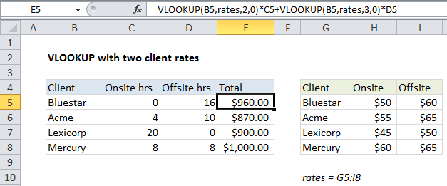
To lookup two different rates for the same client, and calculate a final charge, you can use a formula based on two VLOOKUP functions.

In the example shown, the formula in E5 is:

=VLOOKUP(B5,rates,2,0)*C5+VLOOKUP(B5,rates,3,0)*D5

where “rates” is the named range G5:I8.

How this formula works

This formula is composed of two lookups for the same client. The first lookup finds the onsite rate for the client in column B and multiplies the result by the number of hours in column C:

=VLOOKUP(B5,rates,2,0)*C5

The second lookup finds the offsite rate for same client and multiplies the result by the number of hours in column D:

VLOOKUP(B5,rates,3,0)*D5

In the final step the two results are added together:

=(50*0)+(60*16)
=960

Post navigation

Previous Post:

COSH function: Description, Usage, Syntax, Examples and Explanation

Next Post:

Excel Data validation require unique number

Leave a Reply Cancel reply

Your email address will not be published. Required fields are marked *

Learn Basic Excel

Ribbon
Workbook
Worksheets
Format Cells
Find & Select
Sort & Filter
Templates
Print
Share
Protect
Keyboard Shortcuts

Categories

  • Charts
  • Data Analysis
  • Data Validation
  • Excel Functions
    • Cube Functions
    • Database Functions
    • Date and Time Functions
    • Engineering Functions
    • Financial Functions
    • Information Functions
    • Logical Functions
    • Lookup and Reference Functions
    • Math and Trig Functions
    • Statistical Functions
    • Text Functions
    • Web Functions
  • Excel VBA
  • Excel Video Tutorials
  • Formatting
  • Grouping
  • Others

Logical Functions

  • SWITCH function example in Excel
  • How to use Excel AND Function
  • How to use Excel NOT Function
  • How to return blank in place of #DIV/0! error in Excel
  • How to use Excel XOR Function

Date Time

  • Display Date is same month in Excel
  • WORKDAY.INTL function: Description, Usage, Syntax, Examples and Explanation
  • How to enter Today’s Date or Static Date and Time in Excel
  • How to calculate most recent day of week in Excel
  • Get days between dates in Excel

Grouping

  • How to randomly assign people to groups in Excel
  • Map inputs to arbitrary values in Excel
  • Group times into unequal buckets in Excel
  • Categorize text with keywords in Excel
  • Map text to numbers in Excel

General

  • How to generate random number between two numbers in Excel
  • Convert column letter to number in Excel
  • Basic text sort formula in Excel
  • Advanced Number Formats in Excel
  • Spell Check in Excel
© 2025 xlsoffice . All Right Reserved. | Teal Smiles | Abbreviations And Their Meaning