Skip to content
Free Excel Tutorials
  • Home
  • Excel For Beginners
  • Excel Intermediate
  • Advanced Excel For Experts

Data Analysis

  • How to Create Area Chart in Excel
  • How to Create Column Chart in Excel
  • Move chart to a separate worksheet in Excel
  • How to create Gauge Chart in Excel
  • Number and Text Filters Examples in Excel

References

  • How to use Excel INDIRECT Function
  • How to get relative row numbers in a range in Excel
  • How to use Excel ROWS Function
  • How to use Excel OFFSET function
  • Count rows with at least n matching values

Data Validations

  • Excel Data validation must begin with
  • Excel Data validation no punctuation
  • Excel Data validation date in next 30 days
  • How To Create Drop-down List in Excel
  • Prevent invalid data entering in specific cells

Get address of lookup result in Excel

by

This tutorial shows how to Get address of lookup result in Excel using the example below;

Formula

=CELL("address",INDEX(range,row,col))

Explanation

To get the address of a lookup result derived with INDEX, you can use the CELL function.

Worked Example:   Convert column number to letter in Excel

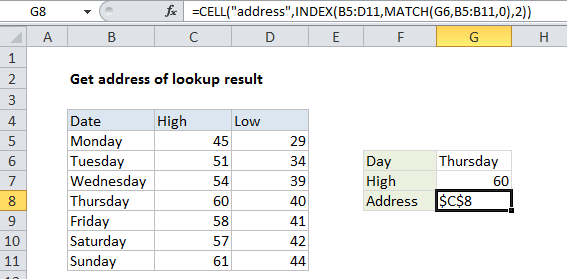
In the example shown, the formula in cell G8 is:

=CELL("address",INDEX(B5:D11,MATCH(G6,B5:B11,0),2))

Which returns an address of $C$8, the address of the cell returned by INDEX.

Worked Example:   Get column name from index in Excel Table

How this formula works

Although INDEX normally displays the value of a cell at a given index, underneath it actually returns a reference.

Worked Example:   Basic INDEX MATCH approximate in Excel

By wrapping INDEX in the ADDRESS function, you can see the address of the cell returned by the lookup.

Post navigation

Previous Post:

Weighted average in Excel

Next Post:

Win loss points calculation in Excel

Leave a Reply Cancel reply

Your email address will not be published. Required fields are marked *

Learn Basic Excel

Ribbon
Workbook
Worksheets
Format Cells
Find & Select
Sort & Filter
Templates
Print
Share
Protect
Keyboard Shortcuts

Categories

  • Charts
  • Data Analysis
  • Data Validation
  • Excel Functions
    • Cube Functions
    • Database Functions
    • Date and Time Functions
    • Engineering Functions
    • Financial Functions
    • Information Functions
    • Logical Functions
    • Lookup and Reference Functions
    • Math and Trig Functions
    • Statistical Functions
    • Text Functions
    • Web Functions
  • Excel VBA
  • Excel Video Tutorials
  • Formatting
  • Grouping
  • Others

Logical Functions

  • SWITCH function example in Excel
  • TRUE function: Description, Usage, Syntax, Examples and Explanation
  • XOR function: Description, Usage, Syntax, Examples and Explanation
  • How to use Excel AND Function
  • How to use Excel FALSE Function

Date Time

  • Convert Excel time to Unix time in Excel
  • Calculate retirement date in Excel
  • Convert date to text in Excel
  • How to calculate workdays per month in Excel
  • Sum through n months in Excel

Grouping

  • Calculate conditional mode with criteria in Excel
  • Group arbitrary text values in Excel
  • If cell contains one of many things in Excel
  • How to randomly assign people to groups in Excel
  • Map text to numbers in Excel

General

  • Check if range contains a value not in another range in Excel
  • Hide and Unhide Columns or Rows in Excel
  • Cell References: Relative, Absolute and Mixed Referencing Examples
  • How to get amount with percentage in Excel
  • How to calculate percent variance in Excel
© 2023 xlsoffice . All Right Reserved. | Teal Smiles | Abbreviations And Their Meaning