Sum Largest Numbers using LARGE function in Excel

LARGE function example shows you how to create an array formula that sums the largest numbers in a range.

Syntax:
LARGE(array, k)

Returns the k-th largest value in a data set.  You can use LARGE to return the highest, runner-up, or third-place score.

For example,

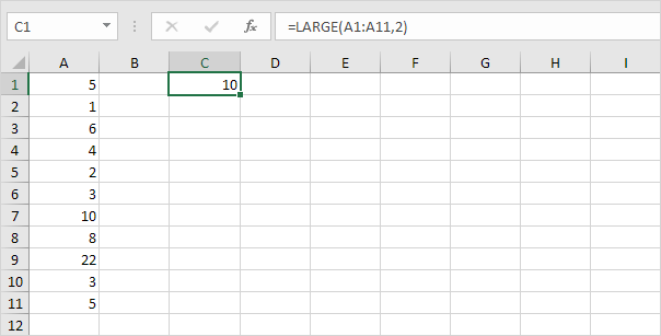
1. Find the second to largest number, use the following function.

2. To sum the 4 largest numbers (don’t be overwhelmed), add the SUM function and replace 2 with {1,2,3,4}.

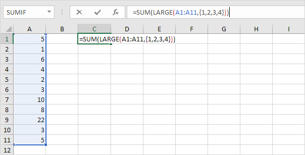
3. Finish by pressing CTRL + SHIFT + ENTER.

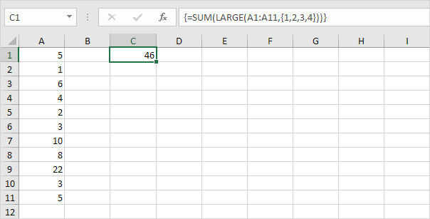
Note: The formula bar indicates that this is an array formula by enclosing it in curly braces {}. Do not type these yourself. They will disappear when you edit the formula.

Explanation: The range (array constant) created by the LARGE function is stored in Excel’s memory, not in a range. The array constant looks as follows.

{22,10,8,6}

This array constant is used as an argument for the SUM function, giving a result of 46.