Vlookup Examples in Excel

The VLOOKUP function is one of the most popular functions in Excel. This chapter contains many easy to follow VLOOKUP examples for Exact Match, Approximate Match, Right Lookup, First Match, Case-insensitive, Multiple Criteria, #N/A error  and  Multiple Lookup Tables.

Exact Match

Most of the time you are looking for an exact match when you use the VLOOKUP function in Excel. Let’s take a look at the arguments of the VLOOKUP function.

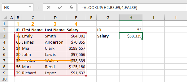
1. The VLOOKUP function below looks up the value 53 (first argument) in the leftmost column of the red table (second argument).

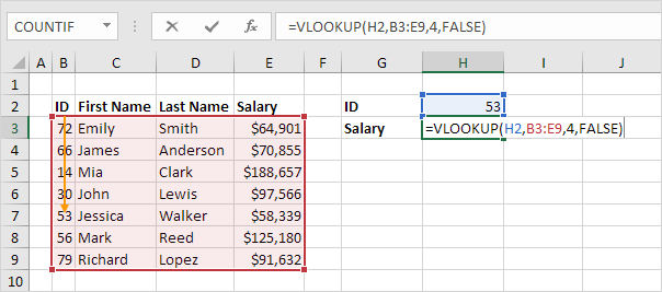
2. The value 4 (third argument) tells the VLOOKUP function to return the value in the same row from the fourth column of the red table.

Note: the Boolean FALSE (fourth argument) tells the VLOOKUP function to return an exact match. If the VLOOKUP function cannot find the value 53 in the first column, it will return a #N/A error.

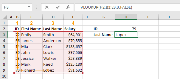
3. Here’s another example. Instead of returning the salary, the VLOOKUP function below returns the last name (third argument is set to 3) of ID 79.

Approximate Match

Let’s take a look at an example of the VLOOKUP function in approximate match mode (fourth argument set to TRUE).

1. The VLOOKUP function below looks up the value 85 (first argument) in the leftmost column of the red table (second argument). There’s just one problem. There’s no value 85 in the first column.

2. Fortunately, the Boolean TRUE (fourth argument) tells the VLOOKUP function to return an approximate match. If the VLOOKUP function cannot find the value 85 in the first column, it will return the largest value smaller than 85. In this example, this will be the value 80.

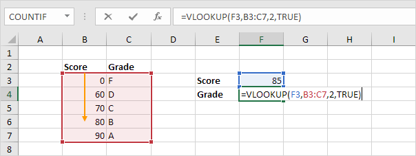
3. The value 2 (third argument) tells the VLOOKUP function to return the value in the same row from the second column of the red table.

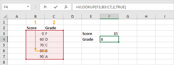
Note: always sort the leftmost column of the red table in ascending order if you use the VLOOKUP function in approximate match mode (fourth argument set to TRUE).

Right Lookup

The VLOOKUP function always looks up a value in the leftmost column of a table and returns the corresponding value from a column to the right.

1. For example, the VLOOKUP function below looks up the first name and returns the last name.

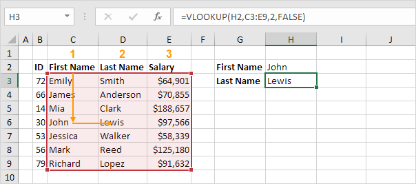
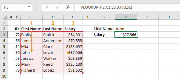
2. If you change the column index number (third argument) to 3, the VLOOKUP function looks up the first name and returns the salary.

Note: in this example, the VLOOKUP function cannot lookup the first name and return the ID. The VLOOKUP function only looks to the right. No worries, you can use the INDEX and the MATCH function in Excel to perform a left lookup.

First Match

If the leftmost column of the table contains duplicates, the VLOOKUP function matches the first instance. For example, take a look at the VLOOKUP function below.

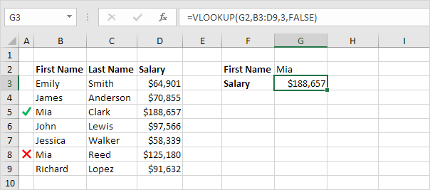
Explanation: the VLOOKUP function returns the salary of Mia Clark, not Mia Reed.

Case-insensitive

The VLOOKUP function in Excel performs a case-insensitive lookup. For example, the VLOOKUP function below looks up MIA (cell G2) in the leftmost column of the table.

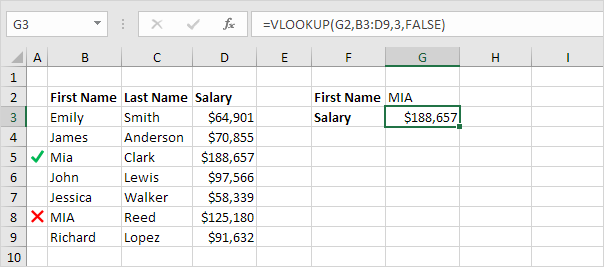
Explanation: the VLOOKUP function is case-insensitive so it looks up MIA or Mia or mia or miA, etc. As a result, the VLOOKUP function returns the salary of Mia Clark (first instance). You can use the INDEX, MATCH and the EXACT function in Excel to perform a case-sensitive lookup.

Multiple Criteria

Do you want to look up a value based on multiple criteria? Use the INDEX and the MATCH function in Excel to perform a two-column lookup.

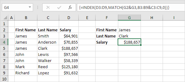
Note: the array formula above looks up the salary of James Clark, not James Smith, not James Anderson.

#N/A error

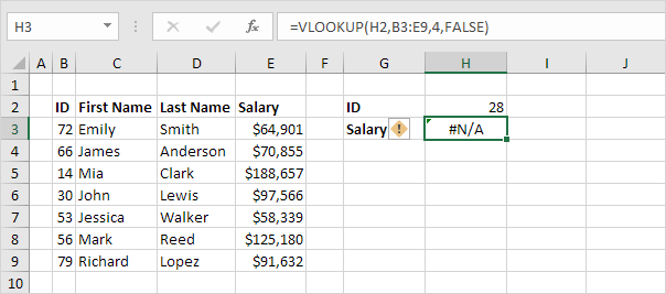
If the VLOOKUP function cannot find a match, it returns a #N/A error.

1. For example, the VLOOKUP function below cannot find the value 28 in the leftmost column.

2. If you like, you can use the IFNA function to replace the #N/A error with a friendly message.

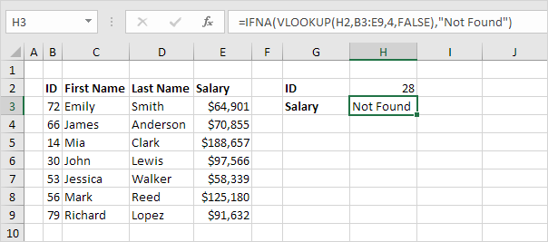
Note: the IFNA function was introduced in Excel 2013. If you’re using Excel 2010 or Excel 2007, simply replace IFNA with IFERROR. Remember, the IFERROR function catches other errors as well. For example, the #NAME? error if you accidentally misspell the word VLOOKUP.

Multiple Lookup Tables

When using the VLOOKUP function in Excel, you can have multiple lookup tables. You can use the IF function to check whether a condition is met, and return one lookup table if TRUE and another lookup table if FALSE.

1. Create two named ranges: Table1 and Table2.

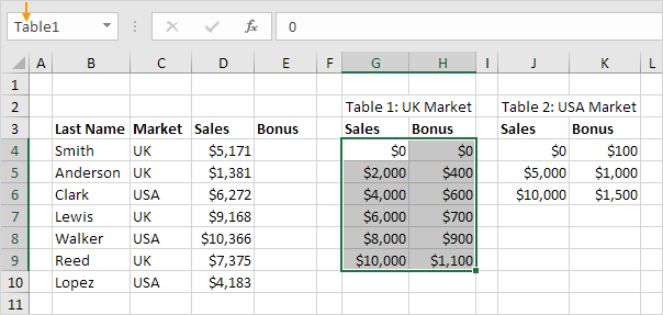
2. Select cell E4 and enter the VLOOKUP function shown below.

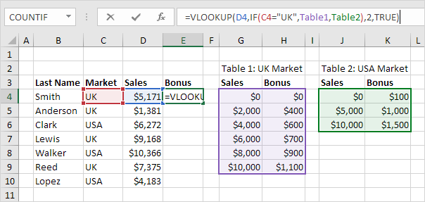
Explanation: the bonus depends on the market (UK or USA) and the sales amount. The second argument of the VLOOKUP function does the trick. If UK, the VLOOKUP function uses Table1, if USA, the VLOOKUP function uses Table2. Set the fourth argument of the VLOOKUP function to TRUE to return an approximate match.

3. Press Enter.

4. Select cell E4, click on the lower right corner of cell E4 and drag it down to cell E10.

Note: for example, Walker receives a bonus of $1,500. Because we’re using named ranges, we can easily copy this VLOOKUP function to the other cells without worrying about cell references.