Calculate payment for a loan in Excel

To calculate a loan payment amount, given an interest rate, the loan term, and the loan amount, you can use the PMT function.

Formula

=PMT(rate,periods,-amount)

Explanation

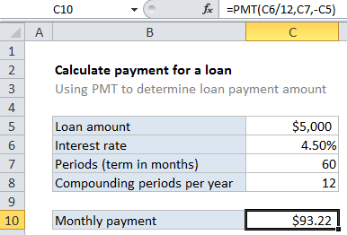
In the example shown, the formula in C10 is:

=PMT(C6/12,C7,-C5)

How this formula works

Loans have four primary components: the amount, the interest rate, the number of periodic payments (the loan term) and a payment amount per period. You can use the PMT function to get the payment when you have the other 3 components.

For this example, we want to find the payment for a $5000 loan with a 4.5% interest rate, and a term of 60 months. To do this, we configure the PMT function as follows:

rate – The interest rate per period. We divide the value in C6 by 12 since 4.5% represents annual interest, and we need the periodic interest.

nper – the number of periods comes from cell C7; 60 monthly periods for a 5 year loan.

pv – the loan amount comes from C5. We use the minus operator to make this value negative, since a loan represents money owed.

With these inputs, the PMT function returns 93.215, rounded to $92.22 in the example using the currency number format.