
Skip to content
Free Excel Tutorials
  • Home
  • Excel For Beginners
  • Excel Intermediate
  • Advanced Excel For Experts

Data Analysis

  • Excel Frequency Function Example
  • Example of COUNTIFS with variable table column in Excel
  • Conflicting Multiple Conditional Formatting Rules in Excel
  • How To Insert and Customize Sparklines in Excel
  • Filter Data Based on Date in Excel

References

  • Extract all partial matches in Excel
  • Basic INDEX MATCH approximate in Excel
  • Extract data with helper column in Excel
  • CHOOSE function: Description, Usage, Syntax, Examples and Explanation
  • How to reference named range different sheet in Excel

Data Validations

  • Excel Data validation only dates between
  • Excel Data validation must begin with
  • Excel Data validation require unique number
  • Excel Data validation unique values only
  • Excel Data validation allow uppercase only

Convert date to Julian format in Excel

by

This tutorial shows how to Convert date to Julian format in Excel using example below.

If you need to convert a date to a Julian date format in Excel, you can do so by building a formula that uses the TEXT, YEAR, and DATE functions.

Formula

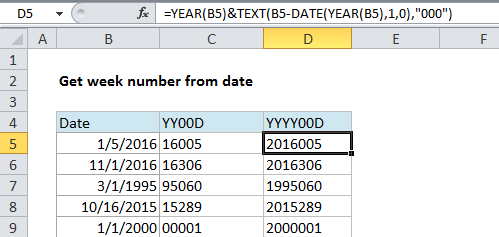
=YEAR(date)&TEXT(date-DATE(YEAR(date),1,0),"000")
How-to-Convert-date-to-Julian-format-in-Excel-excel-tutorials-xlsoffice

Explanation

Background

“Julian date format” refers to a format where the year value of a date is combined with the “ordinal day for that year” (i.e. 14th day, 100th day, etc.) to form a date stamp.

There are several variations. A date in this format may include a 4-digit year (yyyy) or a two-digit year (yy) and the day number may or may not be padded with zeros to always use 3 digits. For example, for the date January 21, 2017, you might see:

1721 // YYD
201721 //YYYYD
2017021 // YYYYDDD

Solution

For a two-digit year + a day number without padding use:

=TEXT(B5,"yy")&B5-DATE(YEAR(B5),1,0)

For a two-digit year + a day number padded with zeros to 3 places:

=TEXT(B5,"yy")&TEXT(B5-DATE(YEAR(B5),1,0),"000")

For a four-digit year + a day number padded with zeros to 3 places:

=YEAR(B5)&TEXT(B5-DATE(YEAR(B5),1,0),"000")

How this formula works

This formula builds the final result in 2 parts, joined by concatenation with the ampersand (&) operator.

On the left of the ampersand, we generate the year value. To extract a 2-digit year, we can use the TEXT function, which can apply a number format inside a formula:

TEXT(B5,"yy")

To extract a full year, use the YEAR function:

YEAR(B5)

On the right side of the ampersand we need to figure out the day of year. We do this by subtracting the last day of the previous year from the date we are working with. Because dates are just serial numbers, this will give us the “nth” day of year.

To get the last day of year of the previous year, we use the DATE function. When you give DATE a year and month value, and a zero for day, you get the last day of the previous month. So:

B5-DATE(YEAR(B5),1,0)

gives us the last day of the previous year, which is December 31, 2015 in the example.

Now we need to pad the day value with zeros. Again, we can use the TEXT function:

TEXT(B5-DATE(YEAR(B5),1,0),"000")

Reverse Julian date

If you need to convert a Julian date back to a regular date, you can use a formula that parses Julian date and runs it through the date function with a month of 1 and day equal to the “nth” day. For example, this would create a date from a yyyyddd Julian date like 1999143.

=DATE(LEFT(A1,4),1,RIGHT(A1,3)) // for yyyyddd

If you just have a day number (e.g. 100, 153, etc.), you can hard-code the year and insert the day this:

=DATE(2016,1,A1)

Where A1 contains the day number. This works because the DATE function knows how to adjust for values that are out of range.

Post navigation

Previous Post:

DECIMAL function: Description, Usage, Syntax, Examples and Explanation

Next Post:

AVERAGE function: Description, Usage, Syntax, Examples and Explanation

Leave a Reply Cancel reply

Your email address will not be published. Required fields are marked *

Learn Basic Excel

Ribbon
Workbook
Worksheets
Format Cells
Find & Select
Sort & Filter
Templates
Print
Share
Protect
Keyboard Shortcuts

Categories

  • Charts
  • Data Analysis
  • Data Validation
  • Excel Functions
    • Cube Functions
    • Database Functions
    • Date and Time Functions
    • Engineering Functions
    • Financial Functions
    • Information Functions
    • Logical Functions
    • Lookup and Reference Functions
    • Math and Trig Functions
    • Statistical Functions
    • Text Functions
    • Web Functions
  • Excel VBA
  • Excel Video Tutorials
  • Formatting
  • Grouping
  • Others

Logical Functions

  • How to return blank in place of #DIV/0! error in Excel
  • SWITCH function example in Excel
  • Invoice status with nested if in Excel
  • How to use Excel OR Function
  • TRUE function: Description, Usage, Syntax, Examples and Explanation

Date Time

  • Calculate expiration date in Excel
  • EDATE function: Description, Usage, Syntax, Examples and Explanation
  • Display the current date in Excel
  • Add business days to date in Excel
  • Get days between dates ignoring years in Excel

Grouping

  • Group numbers at uneven intervals in Excel
  • How to randomly assign people to groups in Excel
  • Group numbers with VLOOKUP in Excel
  • Calculate conditional mode with criteria in Excel
  • Map inputs to arbitrary values in Excel

General

  • Subtotal invoices by age in Excel
  • How to get Excel workbook path only
  • How to calculate percent sold in Excel
  • Convert column number to letter in Excel
  • How to calculate percent of students absent in Excel
© 2026 xlsoffice . All Right Reserved. | Teal Smiles | Abbreviations And Their Meaning