Data Series in Excel

A row or column of numbers that are plotted in a chart is called a data series. You can plot one or more data series in a chart.

To create a column chart, execute the following steps.

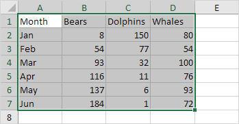
1. Select the range A1:D7.

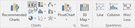
2. On the Insert tab, in the Charts group, click the Column symbol.

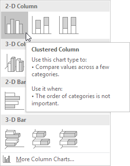
3. Click Clustered Column.

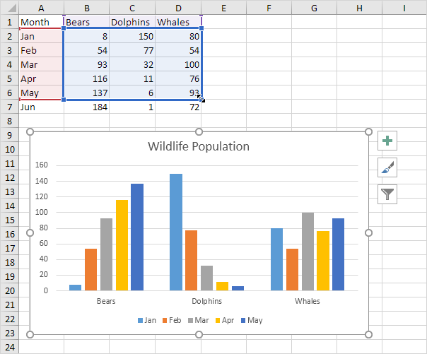
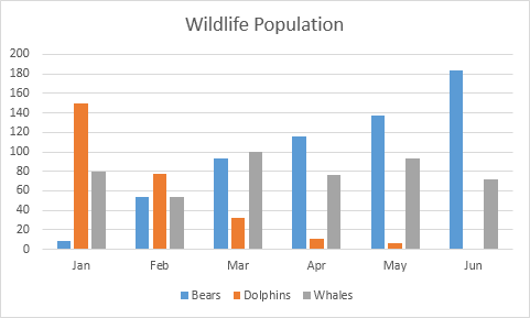
Result:

Select Data Source

To launch the Select Data Source dialog box, execute the following steps.

1. Select the chart. Right click, and then click Select Data.

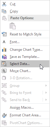
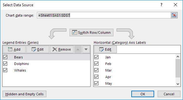
The Select Data Source dialog box appears.

2. You can find the three data series (Bears, Dolphins and Whales) on the left and the horizontal axis labels (Jan, Feb, Mar, Apr, May and Jun) on the right.

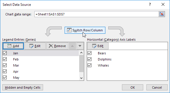
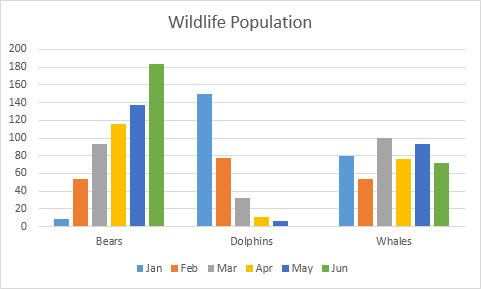
Switch Row/Column

If you click Switch Row/Column, you’ll have 6 data series (Jan, Feb, Mar, Apr, May and Jun) and three horizontal axis labels (Bears, Dolphins and Whales).

Result:

Add, Edit, Remove and Move

You can use the Select Data Source dialog box to add, edit, remove and move data series, but there’s a quicker way.

1. Select the chart.

2. Simply change the range on the sheet.

Result: