Skip to content
Free Excel Tutorials
  • Home
  • Excel For Beginners
  • Excel Intermediate
  • Advanced Excel For Experts

Data Analysis

  • Example of COUNTIFS with variable table column in Excel
  • Reverse List in Excel
  • Get column name from index in Excel Table
  • How To Remove Duplicates In Excel Column Or Row?
  • Subtotal function in Excel

References

  • Get nth match with INDEX / MATCH in Excel
  • VLOOKUP function: Description, Usage, Syntax, Examples and Explanation
  • CHOOSE function: Description, Usage, Syntax, Examples and Explanation
  • How to reference named range different sheet in Excel
  • Count rows with at least n matching values

Data Validations

  • Excel Data validation with conditional list
  • Excel Data validation specific characters only
  • Prevent invalid data entering in specific cells
  • Excel Data validation must begin with
  • Excel Data validation require unique number

Create Scatter Chart in Excel

by

Use a scatter chart (XY chart) to show scientific XY data. Scatter charts are often used to find out if there’s a relationship between variable X and Y.

Straight Lines

To create a scatter chart, execute the following steps.

1. Select the range A1:D22.
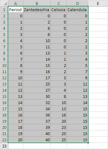
2. On the Insert tab, in the Charts group, click the Scatter symbol.

3. Click Scatter with Straight Lines.
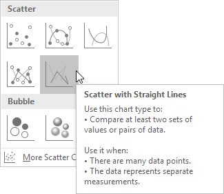
Note: also see the subtype Scatter with Smooth Lines.

Result:

Note: we added a horizontal and vertical axis title. The horizontal axis of a scatter chart is a value axis, so you have more axis scaling options (the same as a vertical axis which always is a value axis).

Only Markers

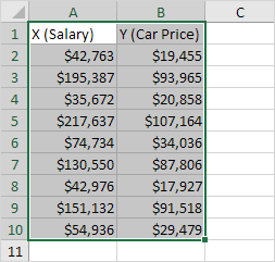
To find out if there is a relationship between X (a person’s salary) and Y (his/her car price), execute the following steps.

1. Select the range A1:B10.
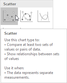
2. On the Insert tab, in the Charts group, click the Scatter symbol.

3. Click Scatter.
Result:

Note: we added a trendline to clearly see the relationship between these two variables.

Post navigation

Previous Post:

VLOOKUP without #N/A error in Excel

Next Post:

Manipulating text strings using Left, Mid, Right, Len, Substitute in Excel

Leave a Reply Cancel reply

Your email address will not be published. Required fields are marked *

Learn Basic Excel

Ribbon
Workbook
Worksheets
Format Cells
Find & Select
Sort & Filter
Templates
Print
Share
Protect
Keyboard Shortcuts

Categories

  • Charts
  • Data Analysis
  • Data Validation
  • Excel Functions
    • Cube Functions
    • Database Functions
    • Date and Time Functions
    • Engineering Functions
    • Financial Functions
    • Information Functions
    • Logical Functions
    • Lookup and Reference Functions
    • Math and Trig Functions
    • Statistical Functions
    • Text Functions
    • Web Functions
  • Excel VBA
  • Excel Video Tutorials
  • Formatting
  • Grouping
  • Others

Logical Functions

  • How to use Excel NOT Function
  • TRUE function: Description, Usage, Syntax, Examples and Explanation
  • How to use Excel XOR Function
  • XOR function: Description, Usage, Syntax, Examples and Explanation
  • Extract multiple matches into separate rows in Excel

Date Time

  • Add business days to date in Excel
  • WEEKDAY function: Description, Usage, Syntax, Examples and Explanation
  • Convert text to date in Excel
  • Get day from date in Excel
  • Display Date is same month in Excel

Grouping

  • How to randomly assign people to groups in Excel
  • Group numbers with VLOOKUP in Excel
  • Running count group by n size in Excel
  • Group times into unequal buckets in Excel
  • Map inputs to arbitrary values in Excel

General

  • Basic error trapping example in Excel
  • How to Delete Cells, Row and Rows in Excel
  • Excel Operators
  • Select, Insert, Rename, Move, Delete Worksheets in Excel
  • How to get amount with percentage in Excel
© 2025 xlsoffice . All Right Reserved. | Teal Smiles | Abbreviations And Their Meaning