
Skip to content
Free Excel Tutorials
  • Home
  • Excel For Beginners
  • Excel Intermediate
  • Advanced Excel For Experts

Data Analysis

  • How to create a Histogram in Excel
  • How To Create Pareto Chart in Excel
  • Example of COUNTIFS with variable table column in Excel
  • How to calculate current stock or inventory in Excel
  • Conflicting Multiple Conditional Formatting Rules in Excel

References

  • Basic INDEX MATCH approximate in Excel
  • Left Lookup in Excel
  • Create hyperlink with VLOOKUP in Excel
  • How to use Excel MMULT Function
  • Extract data with helper column in Excel

Data Validations

  • Excel Data validation must begin with
  • Excel Data validation with conditional list
  • Excel Data validation unique values only
  • Excel Data validation exists in list
  • How To Create Drop-down List in Excel

Superscript and Subscript in Excel

by

Superscript or Subscript generally is a number, figure, symbol, or indicator that is smaller than the normal line of type and is set slightly below it (subscript) or above it (superscript).

It’s easy to format a character as superscript  or subscript in Excel.

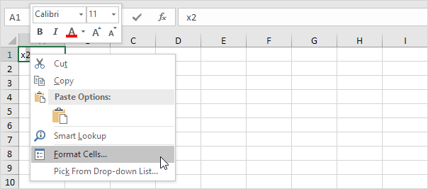
1. For example, double click cell A1.

2. Select the value 2.

3. Right click, and then click Format Cells (or press Ctrl + 1).
The ‘Format Cells’ dialog box appears.

4. On the Font tab, under Effects, click Superscript.
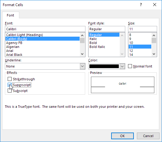

5. Click OK.

Result:

6. Needless to say, a superscript effect cannot return a result. To square a number, use a formula like this:

Note: to insert a caret ^ symbol, press SHIFT + 6.

7. To format a character as subscript (slightly below the baseline), repeat steps 1-5 but at step 4 click Subscript.

Result:

8. Did you know that you can also insert equations in Excel? On the Insert tab, in the Symbols group, click Equation.
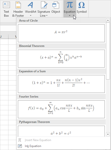
Note: equations in Excel are floating objects and do not return results.

Post navigation

Previous Post:

COSH function: Description, Usage, Syntax, Examples and Explanation

Next Post:

Excel Data validation require unique number

Leave a Reply Cancel reply

Your email address will not be published. Required fields are marked *

Learn Basic Excel

Ribbon
Workbook
Worksheets
Format Cells
Find & Select
Sort & Filter
Templates
Print
Share
Protect
Keyboard Shortcuts

Categories

  • Charts
  • Data Analysis
  • Data Validation
  • Excel Functions
    • Cube Functions
    • Database Functions
    • Date and Time Functions
    • Engineering Functions
    • Financial Functions
    • Information Functions
    • Logical Functions
    • Lookup and Reference Functions
    • Math and Trig Functions
    • Statistical Functions
    • Text Functions
    • Web Functions
  • Excel VBA
  • Excel Video Tutorials
  • Formatting
  • Grouping
  • Others

Logical Functions

  • How to return blank in place of #DIV/0! error in Excel
  • How to use Excel XOR Function
  • How to use Excel OR Function
  • FALSE function: Description, Usage, Syntax, Examples and Explanation
  • SWITCH function example in Excel

Date Time

  • YEAR function: Description, Usage, Syntax, Examples and Explanation
  • Convert Excel time to decimal minutes
  • TIME function: Description, Usage, Syntax, Examples and Explanation
  • TIMEVALUE function: Description, Usage, Syntax, Examples and Explanation
  • EOMONTH function: Description, Usage, Syntax, Examples and Explanation

Grouping

  • Categorize text with keywords in Excel
  • Running count group by n size in Excel
  • How to randomly assign data to groups in Excel
  • Group arbitrary text values in Excel
  • Group times into 3 hour buckets in Excel

General

  • How to calculate profit margin percentage in Excel
  • AutoFit Column Width, AutoFit Row Height in Excel
  • Freeze and Unfreeze Panes in Excel
  • How to calculate decrease by percentage in Excel
  • Split Cell Content Using Text to Columns in Excel
© 2026 xlsoffice . All Right Reserved. | Teal Smiles | Abbreviations And Their Meaning