Freeze and Unfreeze Panes in Excel

If you have a large table of data in Excel, it can be useful to freeze rows or columns. This way you can keep rows or columns visible while scrolling through the rest of the worksheet.

Freeze Top Row

To freeze the top row, execute the following steps.

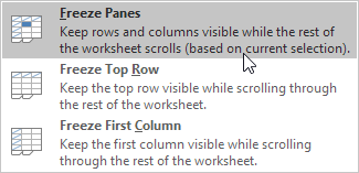
1. On the View tab, in the Window group, click Freeze Panes.

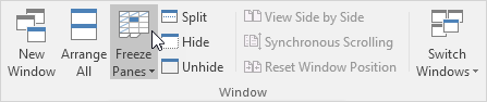
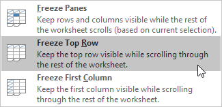
2. Click Freeze Top Row.

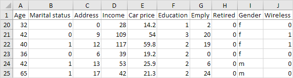
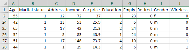
3. Scroll down to the rest of the worksheet.

Result. Excel automatically adds a dark grey horizontal line to indicate that the top row is frozen.

Note: to keep the first column visible while scrolling through the right of the worksheet, click Freeze First Column.

Unfreeze Panes

To unlock all rows and columns, execute the following steps.

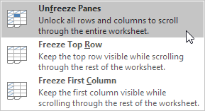
1. On the View tab, in the Window group, click Freeze Panes.

2. Click Unfreeze Panes.

Freeze Panes

To freeze panes, execute the following steps.

1. Select row 3.

2. On the View tab, in the Window group, click Freeze Panes.

3. On the View tab, in the Window group, click Freeze Panes, Freeze Panes.

4. Scroll down to the rest of the worksheet.

Result. All rows above row 3 are frozen.

Note: to keep columns visible while scrolling to the right of the worksheet, select a column and click Freeze panes.

5. Select cell C3 (unfreeze panes first).

6. On the View tab, in the Window group, click Freeze Panes, Freeze Panes.

Result. The region above row 3 and to the left of column C is frozen.