Average last 5 values in columns in Excel

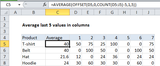
To average the last 5 data values in a range of columns, you can use the AVERAGE function together with the COUNT and OFFSET functions. In the example shown, the formula in F6 is:

=AVERAGE(OFFSET(D5,0,COUNT(D5:J5)-5,1,5))

How this formula works

The OFFSET function can be used to construct dynamic ranges using a starting cell, and given rows, columns, height, and width.

The rows and columns arguments function like “offsets” from the starting reference. The height and width arguments, both optional, determine how many rows and columns the final range includes. We want OFFSET to return a range that begins at the last entry and expands “backwards” so we supply arguments as follows:

reference – the starting reference is D5 – the cell directly to the right of the formula, and the first cell in the range of values we are working with.

rows – we use 0 for the rows argument, because we want to stay in the same row.

columns – for the columns argument, we use the COUNT function to count all values in the range, then subtract 5. This shifts the beginning of the range 5 columns to the left.

height – we use 1 since we want a 1-row range as the final result.

width – we use 5, since we want a final range with 5 columns.

For the formula in C5, OFFSET returns a final range of F5:J5. This goes into the AVERAGE function which returns the average of the 5 values in the range

Less than 5 values

If there are less than 5 values, the formula will return a circular reference error, since the range will extend back into the cell that contains the formula. To prevent this formula, you can adapt the formula as follows:

=AVERAGE(OFFSET(first,0,COUNT(rng)-MIN(N,COUNT(rng)),1,MIN(N,COUNT(rng))))

Here we use the MIN function to “catch” situations where there are less than 5 values, and use the actual count when there are.