Highlight entire rows in Excel

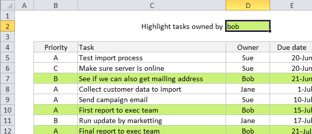
To highlight entire rows with conditional formatting when a value meets specific criteria, use a formula with a mixed reference that locks the column. In the example shown, all rows where the owner is “bob” are highlighted with the following formula applied to B5:E12:

 =$D5="Bob"

Note: CF formulas are entered relative to the “active cell” in the selection, B5 in this case.

How this formula works

When you use a formula to apply conditional formatting, the formula is evaluated relative to the active cell in the selection at the time the rule is created. In this case, the address of the active cell (B5) is used for the row (5) and entered as a mixed address, with column D locked and the row left relative. When the rule is evaluated for each of the 40 cells in B5:E12, the row will change, but the column will not.

Effectively, this causes the rule to ignore values in columns B, C, and E and only test values in column D. When the value in column D for in a given row is “Bob”, the rule will return TRUE for all cells in that row and formatting will be applied to the entire row.

Using other cells as inputs

Note that you don’t have to hard-code any values that might change into the rule. Instead you can use another cell as an “input” cell to hold the value so that you can easily change it later. For example, in this case, you could put “Bob” into cell D2 and then rewrite the formula like so:

=$D5=$D$2

You can then change D2 to any priority you like, and the conditional formatting rule will respond instantly. Just make sure you use an absolute address to keep the input cell address from changing.

Named ranges for a cleaner syntax

Another way to lock references is is to use named ranges, since named ranges are automatically absolute. For example, if you name D2 “owner”, you can rewrite the formula with a cleaner syntax as follows:

=$D5=owner

This makes the formula easier to read and understand.