Average the last 3 numeric values in Excel

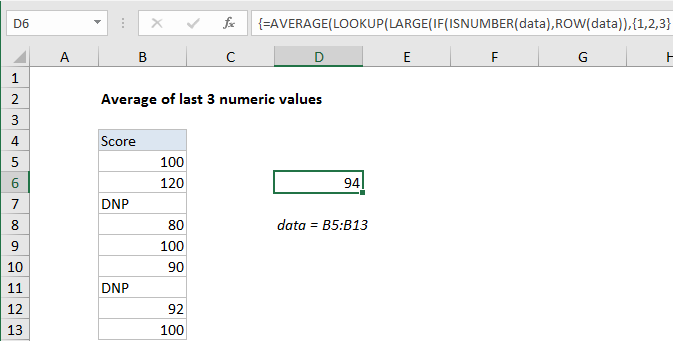
To average the last 3 numeric values in a range, you can use an array formula based on a combination of functions to feed the last n numeric values into the AVERAGE function. In the example shown, the formula in D6 is:

{=AVERAGE(LOOKUP(LARGE(IF(ISNUMBER(data),ROW(data)),{1,2,3}), ROW(data), data))}

where “data” is the named range B5:B13.

Note: this is an array formula, and must be entered with control + shift + enter.

How this formula works

The AVERAGE function will calculate an average of numbers presented in an array, so almost all the work in this formula is to generate an array of the last 3 numeric values in a range. Working from the inside out, the IF function is used to “filter” numeric values:

IF(ISNUMBER(data),ROW(data))

The ISNUMBER function returns TRUE for numeric values, and FALSE for other values (including blanks), and the ROW function returns row numbers, so the result of this operation is an array row numbers that correspond to numeric entries:

{5;6;FALSE;8;9;10;FALSE;12;13}

This array goes into the LARGE function with the array constant {1,2,3} for k. LARGE automatically ignores the FALSE values and returns an array with the largest 3 numbers, which correspond to the last 3 rows with numeric values:

{13,12,10}

This array goes into the LOOKUP function as the lookup value. The lookup array is provided by the ROW function, and the result array is the named range “data”:

LOOKUP({13,12,10}, ROW(data), data))

LOOKUP then returns an array containing corresponding values in “data”, which is fed into AVERAGE:

=AVERAGE({100,92,90})

Handling fewer values

If the number of numeric values drops below 3, this formula will return the #NUM error since LARGE won’t be able to return 3 values as requested. One way to handle this is to replace the hard-coded array constant {1,2,3} with a dynamic array created using INDIRECT like this:

ROW(INDIRECT("1:"&MIN(3,COUNT(data))))

Here, MIN is used  to set the upper limit of the array to 3 or the actual count of numeric values, whichever is smaller.