Skip to content
Free Excel Tutorials
  • Home
  • Excel For Beginners
  • Excel Intermediate
  • Advanced Excel For Experts

Data Analysis

  • Error Bars in Excel
  • How To Remove Duplicates In Excel Column Or Row?
  • Randomize/ Shuffle List in Excel
  • Use Data Form to input, edit and delete records in Excel
  • How to create a Histogram in Excel

References

  • How to use Excel ROWS Function
  • How to get relative row numbers in a range in Excel
  • Lookup entire row in Excel
  • How to use Excel COLUMN Function
  • To count total rows in a range in Excel

Data Validations

  • Excel Data validation allow uppercase only
  • Excel Data validation date in next 30 days
  • Excel Data validation date in specific year
  • Excel Data validation only dates between
  • Excel Data validation don’t exceed total

Sum bottom n values in Excel

by

This tutorial shows how to Sum bottom n values in Excel. You can use a combination of SUMPRODUCT function and SMALL function to get the sum bottom  n values in the example below;

Formula

=SUMPRODUCT(SMALL(range,{1,2,n}))

Explanation

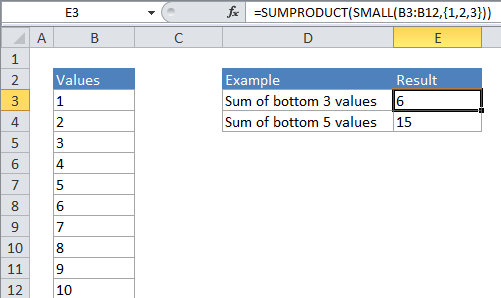
If you need to sum or add the bottom values in a range, you can do so with a formula that uses the SMALL function wrapped inside the SUMPRODUCT function. In the generic form of the formula (above), rng represents a range of cells that contain numeric values and n represents the idea of nth value.

In the example, the active cell contains this formula:

=SUMPRODUCT(SMALL(B4:B13,{1,2,3}))

How this formula works

In its simplest form, SMALL will return the “nth smallest” value in a range. For example, the formula:

=SMALL (A1:A10, 2)

will return the 2nd smallest value in the range A1:A10 which, in the example above, is the number 2.

However, if you supply an “array constant” (e.g. a constant in the form {1,2,3}) to SMALL as the second argument , SMALL will return an array of results instead of a single result. So, the formula:

=SMALL (A1:A10, {1,2,3})

Will return the 1st, 2nd, and 3rd largest value in the range A1:A10. In the example above, where A1:A10 contains the numbers 1-10, the result from SMALL will be the array {1,2,3}. SUMPRODUCT then sums the numbers in this array and returns a total, which is 6.

Using SUMPRODUCT avoids the complexity of entering an array formula, but it is still processing arrays. You can also write an array formula directly using SUM like so:

{=SUM(SMALL(B4:B13,{1,2,3}))}

Note that you must enter this formula as an array formula.

Large N

When N becomes large it becomes tedious to create the array constant by hand – if you want to sum to the bottom 20 or 30 values in a big list of values, typing out an array constant with 20 or 30 items will take a long time. In this case, you can use a shortcut for building the array constant that uses the ROW and INDIRECT functions. For example, if you want to SUM the bottom 20 values in a range called “rng” you can write a formula like this:

=SUMPRODUCT(SMALL(rng,ROW(INDIRECT("1:25"))))

Variable N in another cell

To set up the a formula where N is a variable in another cell, you can concatenate inside INDIRECT. For example, if A1 contains N, you can use:

=SUMPRODUCT(SMALL(range,ROW(INDIRECT("1:"&A1))))

This allows a user to change the value of N directly on the worksheet.

Post navigation

Previous Post:

How to use Excel CHOOSE Function

Next Post:

Customize Ribbon In Excel

Leave a Reply Cancel reply

Your email address will not be published. Required fields are marked *

Learn Basic Excel

Ribbon
Workbook
Worksheets
Format Cells
Find & Select
Sort & Filter
Templates
Print
Share
Protect
Keyboard Shortcuts

Categories

  • Charts
  • Data Analysis
  • Data Validation
  • Excel Functions
    • Cube Functions
    • Database Functions
    • Date and Time Functions
    • Engineering Functions
    • Financial Functions
    • Information Functions
    • Logical Functions
    • Lookup and Reference Functions
    • Math and Trig Functions
    • Statistical Functions
    • Text Functions
    • Web Functions
  • Excel VBA
  • Excel Video Tutorials
  • Formatting
  • Grouping
  • Others

Logical Functions

  • IFS function: Description, Usage, Syntax, Examples and Explanation
  • How to use Excel AND Function
  • Return blank if in Excel
  • How to return blank in place of #DIV/0! error in Excel
  • AND function: Description, Usage, Syntax, Examples and Explanation

Date Time

  • How to calculate project start date based on end date in Excel
  • Get week number from date in Excel
  • Get day from date in Excel
  • DATEVALUE function: Description, Usage, Syntax, Examples and Explanation
  • How to calculate most recent day of week in Excel

Grouping

  • Map inputs to arbitrary values in Excel
  • How to randomly assign data to groups in Excel
  • Group times into 3 hour buckets in Excel
  • Running count group by n size in Excel
  • Categorize text with keywords in Excel

General

  • Automatically fill series of cells in Excel using AutoFill
  • Check if multiple cells have same value with case sensitive in Excel
  • How to generate random number weighted probability in Excel
  • How to generate random date between two dates in Excel
  • How to test a range for numbers in Excel
© 2026 xlsoffice . All Right Reserved. | Teal Smiles | Abbreviations And Their Meaning