Basic INDEX MATCH approximate in Excel

This tutorial shows how to calculate Basic INDEX MATCH approximate in Excel using the example below;

Formula

=INDEX(grades,MATCH(score,scores,1))

Explanation

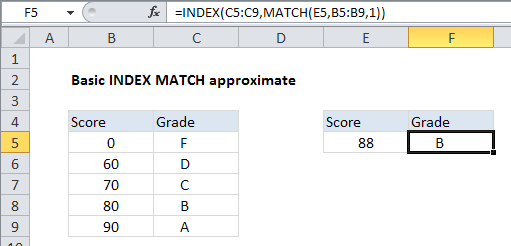
This example shows how to use INDEX and MATCH to retrieve a grade from a table based a given score. This requires an “approximate match”, since it is unlikely that the actual score exists in the table. The formula in cell F5 is:

=INDEX(C5:C9,MATCH(E5,B5:B9,1))

Which returns “B”, the correct grade for a score of 88.

How this formula works

This formula uses MATCH find the correct row for a given score.  MATCH is configured to look for the value in E5 in column B:

MATCH(E5,B5:B9,1)

Note that the last argument is 1 (equivalent to TRUE), which allows MATCH to perform an approximate match on values listed in ascending order. In this configuration, MATCH returns the position of the first value that is less than or equal to the lookup value. In this case, the score is 88, row 4 is returned.

Once MATCH returns 4 we have:

=INDEX(C5:C9,4)

Which causes INDEX to retrieve the value at the 4th row of the range C5:C9, which is “B”.

Note: values in column B must be sorted in ascending order in order for MATCH to return the correct position.