How to Create One and Two Variable Data Tables in Excel

Instead of creating different scenarios, you can create a data table to quickly try out different values for formulas. You can create a one variable data table or a two variable data table.

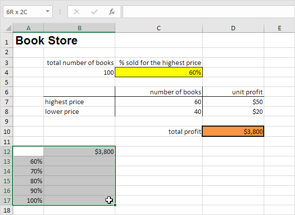
Assume you own a book store and have 100 books in storage. You sell a certain % for the highest price of $50 and a certain % for the lower price of $20. If you sell 60% for the highest price, cell D10 below calculates a total profit of 60 * $50 + 40 * $20 = $3800.

One Variable Data Table

To create a one variable data table, execute the following steps.

1. Select cell B12 and type =D10 (refer to the total profit cell).

2. Type the different percentages in column A.

3. Select the range A12:B17.

We are going to calculate the total profit if you sell 60% for the highest price, 70% for the highest price, etc.

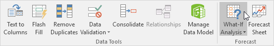
4. On the Data tab, in the Forecast group, click What-If Analysis.

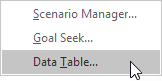
5. Click Data Table.

6. Click in the ‘Column input cell’ box (the percentages are in a column) and select cell C4.

We select cell C4 because the percentages refer to cell C4 (% sold for the highest price). Together with the formula in cell B12, Excel now knows that it should replace cell C4 with 60% to calculate the total profit, replace cell C4 with 70% to calculate the total profit, etc.

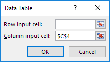
Note: this is a one variable data table so we leave the Row input cell blank.

7. Click OK.

Result.

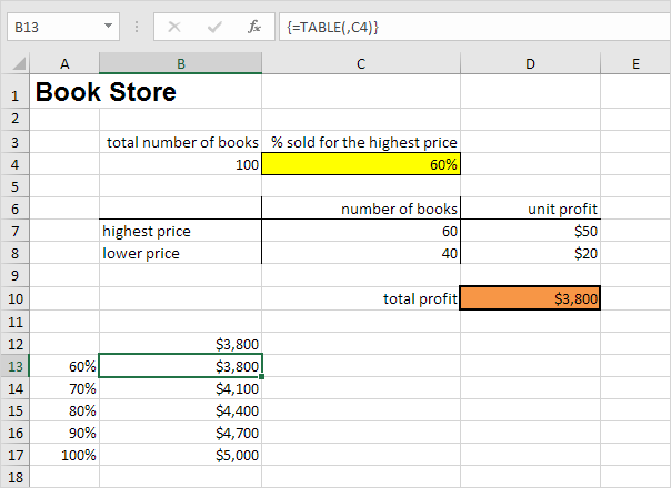
Conclusion: if you sell 60% for the highest price, you obtain a total profit of $3800, if you sell 70% for the highest price, you obtain a total profit of $4100, etc.

Note: the formula bar indicates that the cells contain an array formula. Therefore, you cannot delete a single result. To delete the results, select the range B13:B17 and press Delete.

Two Variable Data Table

To create a two variable data table, execute the following steps.

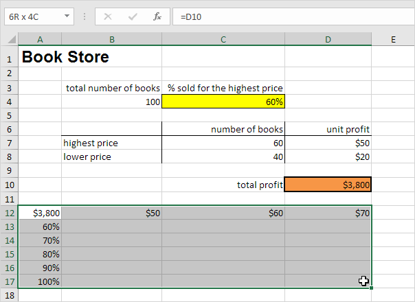
1. Select cell A12 and type =D10 (refer to the total profit cell).

2. Type the different unit profits (highest price) in row 12.

3. Type the different percentages in column A.

4. Select the range A12:D17.

We are going to calculate the total profit for the different combinations of ‘unit profit (highest price)’ and ‘% sold for the highest price’.

5. On the Data tab, in the Forecast group, click What-If Analysis.

6. Click Data Table.

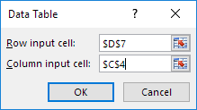
7. Click in the ‘Row input cell’ box (the unit profits are in a row) and select cell D7.

8. Click in the ‘Column input cell’ box (the percentages are in a column) and select cell C4.

We select cell D7 because the unit profits refer to cell D7. We select cell C4 because the percentages refer to cell C4. Together with the formula in cell A12, Excel now knows that it should replace cell D7 with $50 and cell C4 with 60% to calculate the total profit, replace cell D7 with $50 and cell C4 with 70% to calculate the total profit, etc.

9. Click OK.

Result.

Conclusion: if you sell 60% for the highest price, at a unit profit of $50, you obtain a total profit of $3800, if you sell 80% for the highest price, at a unit profit of $60, you obtain a total profit of $5200, etc.

Note: the formula bar indicates that the cells contain an array formula. Therefore, you cannot delete a single result. To delete the results, select the range B13:D17 and press Delete.