Faster VLOOKUP with 2 VLOOKUPS in Excel

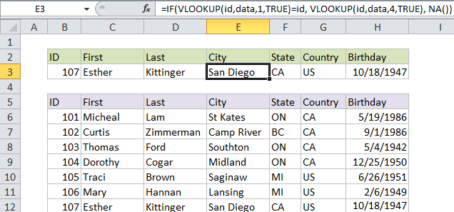
=IF(VLOOKUP(id,data,1,TRUE)=id, VLOOKUP(id,data,col,TRUE), NA())

With large sets of data, exact match VLOOKUP can be painfully slow, but you can make VLOOKUP lightening fast by using two VLOOKUPS, as explained below.

Notes:

1. If you have a smaller set of data, this approach is overkill. Only use it with large data sets when speed really counts.
2. You must sort the data by lookup value in order for this trick to work.
3. This example uses named ranges. If you don’t want to use named ranges use absolute references instead.

Exact-match VLOOKUP is slow

When you use VLOOKUP in “exact match mode” on a large set of data, it can really slow down the calculation time in a worksheet. With, say, 50,000 records, or 100,000 records, calculation can take minutes.

Exact match is set by supplying FALSE or zero as the forth argument:

=VLOOKUP(val,data,col,FALSE)

The reason VLOOKUP in this mode is slow is because it must check every single record in the data set until a match is found. This is sometimes referred to as a linear search.

Approximate-match VLOOKUP is very fast

In approximate-match mode, VLOOKUP is extremely fast. To use approximate-match VLOOKUP, you must sort your data by the first column (the lookup column), then specify TRUE for the 4th argument:

=VLOOKUP(val,data,col,TRUE)

(VLOOKUP defaults to true, which is a scary default, but that’s another story).

With very large sets of data, changing to approximate-match VLOOKUP can mean a dramaticspeed increase.

So, no-brainer, right? Just sort the data, use approximate match, and you’re done.

Not so fast (heh).

The problem with VLOOKUP in “approximate match” mode is this: VLOOKUP won’t display an error if the lookup value doesn’t exist. Worse, the result may look completely normal, even though it’s totally wrong (see examples). Not something you want to explain to your boss.

The solution is to use VLOOKUP twice, both times in approximate match mode:

=IF(VLOOKUP(id,data,1,TRUE)=id, VLOOKUP(id,data,col,TRUE), NA())

How this formula works

The first instance of VLOOKUP simply looks up the lookup value (the id in this example):

=IF(VLOOKUP(id,data,1,TRUE)=id

and returns TRUE only when the lookup value is found. In that case,
the formula runs VLOOKUP again in approximate match mode to retrieve a value from that table:

VLOOKUP(id,data,col,TRUE)

There’s no danger of a missing lookup value, since the first part of the formula already checked to make sure it’s there.

If the lookup value isn’t found, the “value if FALSE” part of the IF function runs, and you can return any value you like. In this example, we use NA() we return an #N/A error, but you could also return a message like “Missing” or “Not found”.

Remember: you must sort the data by lookup value in order for this trick to work.