
Skip to content
Free Excel Tutorials
  • Home
  • Excel For Beginners
  • Excel Intermediate
  • Advanced Excel For Experts

Data Analysis

  • Example of COUNTIFS with variable table column in Excel
  • Use Data Form to input, edit and delete records in Excel
  • Randomize/ Shuffle List in Excel
  • How to calculate average last N values in a table in Excel
  • Get column name from index in Excel Table

References

  • How to use Excel COLUMN Function
  • Count rows that contain specific values in Excel
  • How to calculate two-way lookup VLOOKUP in Excel Table
  • How to use Excel MMULT Function
  • LOOKUP function: Description, Usage, Syntax, Examples and Explanation

Data Validations

  • Prevent invalid data entering in specific cells
  • Excel Data validation only dates between
  • Excel Data validation unique values only
  • Excel Data validation no punctuation
  • How To Create Drop-down List in Excel

Sum matching columns in Excel

by

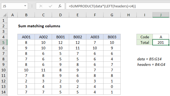
This tutorial shows how to sum matching columns in Excel using the example below;

Formula

=SUMPRODUCT(data*(headers=A1))
Explanation

To sum values in columns by matching matching column headers, you can use a formula based on the SUMPRODUCT function. In the example shown, the formula in J5 is:

=SUMPRODUCT(data*(LEFT(headers)=J4))

where “data” is the named range C5:G14, and “headers” is the named range C4:G4.

The formula sums columns where headers begin with “a” and returns 201.

How this formula works

At the core, this formula relies on the SUMPRODUCT function to sum values in matching columns in the named range “data” C5:G14. If all data were provided to SUMPRODUCT in a single range, the result would be the sum of all values in the range:

=SUMPRODUCT(data) // all data, returns 387

To apply a filter by matching column headers – columns with headers that begin with “A” – we use the LEFT function like this:

LEFT(headers)=J4) // must begin with "a"

This expression returns TRUE if a column header begins with “a”, and FALSE if not. The result is an array:

{TRUE,TRUE,FALSE,FALSE,TRUE,FALSE}

You can see that values 1,2, and 5 correspond to columns that begin with “a”.

Inside SUMPRODUCT, this array is multiplied by “data”. Due to broadcasting, the result is a two-dimensional array like this:

{8,10,0,0,7,0;9,10,0,0,10,0;8,6,0,0,6,0;7,6,0,0,6,0;8,6,0,0,6,0;10,11,0,0,7,0;7,8,0,0,8,0;2,3,0,0,3,0;3,4,0,0,4,0;7,7,0,0,4,0}

If we visualize this array in a table, it’s easy to see that only values in columns that begin with “a” have survived the operation, all other columns are zero. In other words, the filter keeps values of interest and “cancels out” the rest:

A001 A002 B001 B002 A003 B003
8 10 0 0 7 0
9 10 0 0 10 0
8 6 0 0 6 0
7 6 0 0 6 0
8 6 0 0 6 0
10 11 0 0 7 0
7 8 0 0 8 0
2 3 0 0 3 0
3 4 0 0 4 0
7 7 0 0 4 0

With only a single array to process, SUMPRODUCT returns the sum of all values, 201.

Post navigation

Previous Post:

How to use Excel CHOOSE Function

Next Post:

Customize Ribbon In Excel

Leave a Reply Cancel reply

Your email address will not be published. Required fields are marked *

Learn Basic Excel

Ribbon
Workbook
Worksheets
Format Cells
Find & Select
Sort & Filter
Templates
Print
Share
Protect
Keyboard Shortcuts

Categories

  • Charts
  • Data Analysis
  • Data Validation
  • Excel Functions
    • Cube Functions
    • Database Functions
    • Date and Time Functions
    • Engineering Functions
    • Financial Functions
    • Information Functions
    • Logical Functions
    • Lookup and Reference Functions
    • Math and Trig Functions
    • Statistical Functions
    • Text Functions
    • Web Functions
  • Excel VBA
  • Excel Video Tutorials
  • Formatting
  • Grouping
  • Others

Logical Functions

  • IF with wildcards in Excel
  • How to use IFS function in Excel
  • Invoice status with nested if in Excel
  • XOR function: Description, Usage, Syntax, Examples and Explanation
  • IF, AND, OR and NOT Functions Examples in Excel

Date Time

  • Steps to create Dynamic calendar grid in Excel
  • Get days between dates ignoring years in Excel
  • Display Days until expiration date in Excel
  • Calculate total hours that fall between two times in Excel
  • Convert decimal hours to Excel time

Grouping

  • Calculate conditional mode with criteria in Excel
  • Running count group by n size in Excel
  • Group arbitrary text values in Excel
  • Map inputs to arbitrary values in Excel
  • Map text to numbers in Excel

General

  • Lock Cells in a Worksheet Excel
  • Customize Ribbon In Excel
  • How to add sequential row numbers to a set of data in Excel
  • How to increase by percentage in Excel
  • 3D SUMIF for multiple worksheets in Excel
© 2026 xlsoffice . All Right Reserved. | Teal Smiles | Abbreviations And Their Meaning