
Skip to content
Free Excel Tutorials
  • Home
  • Excel For Beginners
  • Excel Intermediate
  • Advanced Excel For Experts

Data Analysis

  • Excel Frequency Function Example
  • How to Use Solver Tool in Excel
  • How to calculate correlation coefficient Correlation in Excel
  • Move chart to a separate worksheet in Excel
  • Example of COUNTIFS with variable table column in Excel

References

  • How to get last row in mixed data with blanks in Excel
  • How to get address of first cell in range in Excel
  • How to reference named range different sheet in Excel
  • How to use Excel VLOOKUP Function
  • How to get first row number in range in Excel

Data Validations

  • Excel Data validation only dates between
  • Excel Data validation exists in list
  • Excel Data validation date in next 30 days
  • Excel Data validation no punctuation
  • Excel Data validation with conditional list

Sum if cells contain an asterisk in Excel

by

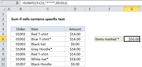
This tutorial shows how to Sum if cells contain an asterisk in Excel using the example below;

Formula

=SUMIF(range,"*~**",sum_range)
Explanation

To sum if cells contain an asterisk, you can use the SUMIF function with the special “escape” character “~”. In the example shown, cell G6 contains this formula:

=SUMIF(C5:C11,"*~**",D5:D11)

This formula sums the amounts in column D when a value in column C contains “*”.

How the formula works

The SUMIF function supports wildcards. An asterisk (*) means “one or more characters”, while a question mark (?) means “any one character”.

These wildcards allow you to create criteria such as “begins with”, “ends with”, “contains 3 characters” and so on.

Because asterisks and question marks are themselves wildcards, if you want to search for these characters specifically, you’ll need to escape them with a tilde (~). The tilde causes Excel to treat the following character literally.

In this case we are using “~*” to match a literal asterisk, but this is surrounded by asterisks on either side, in order to match an asterisk anywhere in the cell. If you just want to match an asterisk at the end of a cell, use: “*~*” for the criteria.

Alternative with SUMIFS

You can also use the SUMIFS function. SUMIFS can handle multiple criteria, and the order of the arguments is different from SUMIF. With SUMIFS, the sum range always comes first in the argument list, followed by range/criteria pairs:

=SUMIFS(D5:D11,C5:C11,"*~**")

Post navigation

Previous Post:

How to use Excel CHOOSE Function

Next Post:

Customize Ribbon In Excel

Leave a Reply Cancel reply

Your email address will not be published. Required fields are marked *

Learn Basic Excel

Ribbon
Workbook
Worksheets
Format Cells
Find & Select
Sort & Filter
Templates
Print
Share
Protect
Keyboard Shortcuts

Categories

  • Charts
  • Data Analysis
  • Data Validation
  • Excel Functions
    • Cube Functions
    • Database Functions
    • Date and Time Functions
    • Engineering Functions
    • Financial Functions
    • Information Functions
    • Logical Functions
    • Lookup and Reference Functions
    • Math and Trig Functions
    • Statistical Functions
    • Text Functions
    • Web Functions
  • Excel VBA
  • Excel Video Tutorials
  • Formatting
  • Grouping
  • Others

Logical Functions

  • OR function Examples in Excel
  • Not Equal To ‘<>‘ operator in Excel
  • Nested IF function example in Excel
  • Extract multiple matches into separate rows in Excel
  • How to use Excel TRUE Function

Date Time

  • Assign points based on late time in Excel
  • Steps to create Dynamic calendar grid in Excel
  • How to calculate working days left in month in Excel
  • DAY function: Description, Usage, Syntax, Examples and Explanation
  • Convert date string to date time in Excel

Grouping

  • Group numbers with VLOOKUP in Excel
  • How to randomly assign data to groups in Excel
  • Group arbitrary text values in Excel
  • Calculate conditional mode with criteria in Excel
  • Group times into 3 hour buckets in Excel

General

  • Excel Autofill Cell Ranges, Copy, Paste
  • Find Most Frequently Occurring Word in Excel Worksheet
  • Basic error trapping example in Excel
  • How to calculate percentage discount in Excel
  • How to calculate percent of students absent in Excel
© 2026 xlsoffice . All Right Reserved. | Teal Smiles | Abbreviations And Their Meaning