How to Create Running Total (Cumulative Sum) in Excel

A running total changes each time new data is added to a list. This example teaches you how to create a running total (cumulative sum) in Excel.

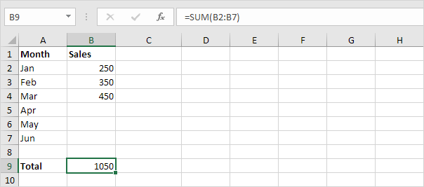
1. Select cell B9 and enter a simple SUM function.

2. Select cell C2 and enter the SUM function shown below.

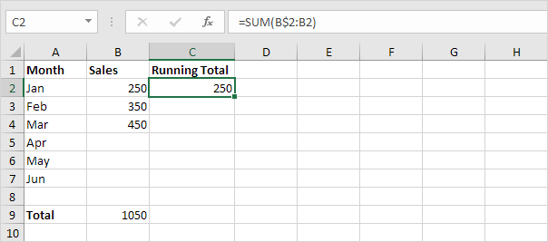
Explanation: the first cell (B$2) in the range reference is a mixed reference. We fixed the reference to row 2 by adding a $ symbol in front of the row number. The second cell (B2) in the range reference is a normal relative reference.

3. Select cell C2, click on the lower right corner of cell C2 and drag it down to cell C7.

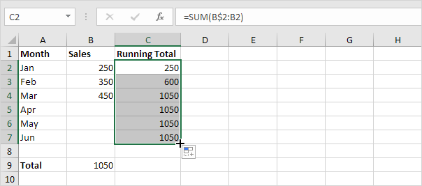
Explanation: when we drag the formula down, the mixed reference (B$2) stays the same, while the relative reference (B2) changes to B3, B4, B5, etc.

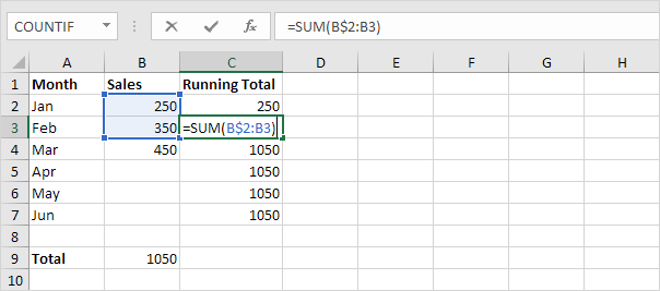
4. For example, take a look at the formula in cell C3.

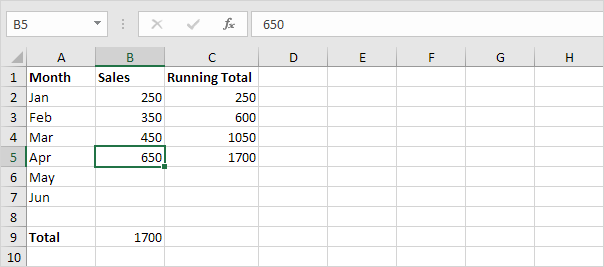
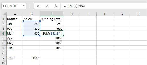
5. For example, take a look at the formula in cell C4.

6. At step 2, enter the IF function shown below (and drag it down to cell C7) to only display a cumulative sum if data has been entered.

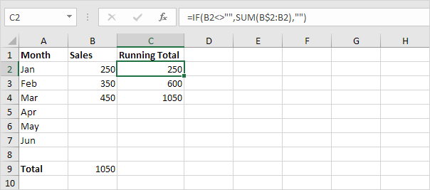
Explanation: if cell B2 is not empty (<> means not equal to), the IF function in cell C2 displays a cumulative sum, else it displays an empty string.

7. Enter the sales in April.