Get location of value in 2D array in Excel
This tutorial shows how to Get location of value in 2D array in Excel using the example below;
Formula
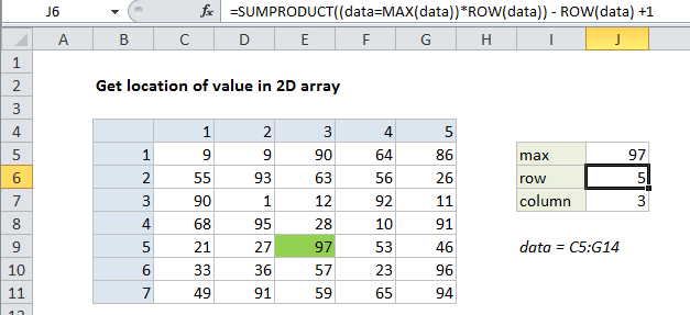
=SUMPRODUCT((data=MAX(data))*ROW(data))-ROW(data)+1
Explanation
To locate the position of a value in a 2D array, you can use the SUMPRODUCT function. In the example shown, the formulas used to locate the row and column numbers of the max value in the array are:
=SUMPRODUCT((data=MAX(data))*ROW(data))-ROW(data)+1
=SUMPRODUCT((data=MAX(data))*COLUMN(data))-COLUMN(data)+1
where “data” is the named range C5:G14.
Note: for this example, we are arbitrarily find the location of the maximum value in the data, but you can replace data=MAX(data) with any other logical test that will isolate a given value. Also note these formulas will fail if there are duplicate values in the array.
How these formula work
To get the row number, the data is compared to the max value, which generates an array of TRUE FALSE results. These are multiplied by the result of ROW (data) which generates and array of row numbers associated with the named range “data”:
=SUMPRODUCT({FALSE,FALSE,FALSE,FALSE,FALSE;FALSE,FALSE,FALSE,FALSE,FALSE;FALSE,FALSE,FALSE,FALSE,FALSE;FALSE,FALSE,FALSE,FALSE,FALSE;FALSE,FALSE,TRUE,FALSE,FALSE;FALSE,FALSE,FALSE,FALSE,FALSE;FALSE,FALSE,FALSE,FALSE,FALSE}*{5;6;7;8;9;10;11})
The multiplication operation causes Excel to coerce the TRUE FALSE values in the first array to 1s and 0s, so we can visualize an intermediate step like this:
=SUMPRODUCT({0,0,0,0,0;0,0,0,0,0;0,0,0,0,0;0,0,0,0,0;0,0,1,0,0;0,0,0,0,0;0,0,0,0,0}*{5;6;7;8;9;10;11})
SUMPRODUCT then returns a result of 9, which corresponds to the 9th row on the worksheet. To get an index relative to the named range “data”, we use:
-ROW(data)+1
The final result is the array {5;4;3;2;1;0;-1}, from which only the first value (5) is displayed.
The formula to determine the column position works in the same way.