Categorize text with keywords in Excel

This tutorial shows how to Categorize text with keywords in Excel using the example below;

Formula

{=INDEX(categories,MATCH(TRUE,ISNUMBER
(SEARCH(keywords,text)),0))}

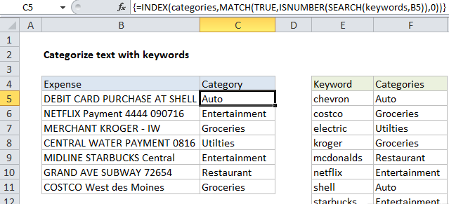
To categorize text using keywords with a “contains” match, you can use the SEARCH function, with help from INDEX and MATCH. In the example shown, the formula in C5 is:

{=INDEX(categories,MATCH(TRUE,
ISNUMBER(SEARCH(keywords,B5)),0))}

where “keywords” is the named range E5:E14, and “categories” is the named range F5:F14.

Note: this is an array formula and must be entered with control + shift  + enter.

How this formula works

At the core, this formula is using the SEARCH function to search cells in column B for every possible keyword in the named range “keywords” (E5:E14):

SEARCH(keywords,B5)

Because we are looking for multiple items (in the named range “keywords”), we’ll get back multiple results like this:

{#VALUE!;#VALUE!;#VALUE!;#VALUE!;

#VALUE!;#VALUE!;24;#VALUE!;#VALUE!;#VALUE!}

The #VALUE! error occurs when SEARCH can’t find the text. When SEARCH does get a match, it returns a number that corresponds to the position of the text inside the cell.

To change these results into a more usable format, we use the ISNUMBER function, which changes all values to TRUE/FALSE like so:

{FALSE;FALSE;FALSE;FALSE;FALSE;FALSE;TRUE;FALSE;FALSE;FALSE}

This array goes into the MATCH function as the lookup_array, with the lookup_value set as TRUE. MATCH then returns the position of the first TRUE it finds in the array (7 in this case) which is provided to INDEX as the row_num:

=INDEX(categories,7)

With categories as the array, and 7 as the row number, INDEX returns “Auto”.

Preventing false matches

One problem with this approach is you may get false matches from substrings that appear inside longer words. For example, if you try to match “dr” you may also find “Andrea”, “drink”, “dry”, etc. since “dr” appears inside these words. This happens because SEARCH automatically does a “contains” match.

For a quick hack, you can add space around the search words (i.e. ” dr “, or “dr “) to avoid catching “dr” in another word. But this will fail if “dr” appears first or last in a cell, or appears with punctuation, etc.

If you need a more accurate solution, one option is to normalize the text first in a helper column, taking care to also add a leading and trailing space. Then you can search for whole words surrounded by spaces.